Inelastic Buckling Theory

Let’s start with classical Euler Buckling, as follows.

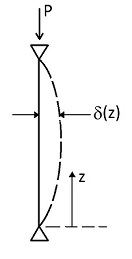
External moment: $P*\delta$
Internal moment: $-EI*\frac{d^2\delta}{dz^2}$

If $P$ is small, $-EI*\frac{d^2\delta}{dz^2}>>P*\delta$ , where we can see that both sides of the equality are dependent on $\delta$ . The column will remain straight until $P$ reaches a critical value. Thus, classical Euler Buckling is associated with instability rather than strength.

$P*\delta-M=0$
OR

(1) $\begin{equation*} P*\delta+EI*\frac{d^2\delta}{dz^2}=0 \end{equation*}$

Eq. 1 has a “+” in anticipation of the solution being a sine function. The second derivative of a sine function has the opposite sign of the function itself, so the two terms of eq. 1 will indeed have opposite signs and will sum to zero.

Eq. 1 is a $2^{nd} Order ODE$ with constant coefficients.
The solution to eq. 1 is:

$\begin{equation*} \delta(z)=A\sin\bigg(\sqrt{\frac{P}{EI}}*z\bigg)+B\cos\bigg(\sqrt{\frac{P}{EI}}*z\bigg) \end{equation*}$

We can employ pin-pin boundary conditions ( $\delta(z=0)=0$ and $\delta(z=L)=0$ ) and see that $0=B$ and $0=A\sin\bigg(\sqrt{\frac{P}{EI}}*L\bigg)$ .
For a nontrivial solution, we need to therefore satisfy $\sin\bigg(\sqrt{\frac{P}{EI}}*L\bigg)=0$ . This is true when $\sqrt{\frac{P}{EI}}*L=0,\pi,2\pi...n\pi$ . The dominant buckling mode for our columns will occur when $\sqrt{\frac{P}{EI}}*L=\pi$ .

So, $P_{cr}=\frac{\pi^2 EI}{L^2}$ , where the subscript “cr” stand for “critical,” and our expression is valid for a pin-pin column that buckles elastically. If “r” = “radius of gyration”= $\sqrt{I/A}$ , then we can write, equivalently, $P_{cr}=\frac{\pi^2 EAr^2}{L^2}=\frac{\pi^2 EA}{(L/r)^2}$ .

A more general expression, that is valid for other boundary conditions, can be written:

(2) $\begin{equation*} P_{cr}=\frac{\pi^2 E}{(KL/r)^2}A=\frac{\pi^2 E I}{(KL)^2} \end{equation*}$

In eq. 2, $K$ is the “effective length factor” or “K-factor” and the quantity $KL/r$ is the “slenderness ratio.”

It is important to know what factors influence the effective length factor, $K$ . Noting that this K-factor is squared in eq. 2, we can see that choosing the wrong $K$ can result in extreme error. Some important factors that influence $K$ include the kind of connection at the bottom and top of the column (e.x. moment connection or steel shear connection), the size of the beam that is intersecting at these locations, as well as whether the structure, as a whole, is “braced.”

For very slender columns, the above equation for column strength is approximately correct. For very short columns, failure will occur via yielding of the entire cross-section, rather than buckling. For most realistic columns (e.x. columns chosen from the AISC Manual that span a typical story height), the limit state will be partial yielding followed by buckling. This limit state is commonly called inelastic buckling and this phenomenon forms the basis for the AISC equations for column compression capacity.

The following derivation, which is adapted from Salmon and Johnson [Salmon], will show where the AISC equations come from.

Let’s consider weak axis inelastic buckling of a wide-flange I-shape. When such a column begins to yield, it will do so in the manner shown in the figure below.

Note in the above Fig that the four flange tips are yielding in compression. The reason for this will be explained shortly (residual stresses).

Our first assumption is to replace the modulus of elasticity, $E$ , which is present in eq. 2, with a reduced value, $E_t$ . The assumption is that this tangent modulus, $E_t$ can be related to $E$ in the following way:

$\begin{equation*} E_t=\overbrace{\frac{I_e}{I}}^{\text{effective}}E \end{equation*}$

Ignoring the contribution of the web to the moment of inertia about the weak axis,
$I=2*\bigg[\frac{1}{12}(\text{base})(\text{height})^3\bigg]=\frac{1}{12}(t_f)b^3*2$
$I_e=\frac{1}{12}(t_f)(2x_0)^3*2$

So, $E_t=\frac{I_e}{I}E=E*\frac{t_f(2x_0)^3}{12}(\frac{12}{t_f b^3})*\frac{2}{2}=E*(\frac{2x_0}{b})^3$

note: A small value of $2x_0$ represents significant yielding within the cross-section. As $2x_0$ approaches zero, $E_t$ does indeed approach zero.

We can now substitute our expression for $E_t$ into eq. 2. The result is:

$\begin{equation*} P_{cr}=\frac{\pi^2 E_t}{(KL/r)^2}A=\frac{\pi^2 E \frac{I_e}{I}}{(KL/r)^2}A=\frac{\pi^2 E (\frac{2x_0}{b})^3}{(KL/r)^2}A=\frac{8\pi^2 E (\frac{x_0}{b})^3}{(KL/r)^2}A \end{equation*}$

(3) $\begin{equation*} F_{cr}=\frac{8\pi^2 E (\frac{x_0}{b})^3}{(KL/r)^2} \end{equation*}$

According to eq. 3, we can say that the critical buckling stress, $F_{cr}$ , is a function of two variables, $\frac{x_0}{b}$ , and $\frac{KL}{r}$ . In other words, the critical buckling stress depends on how much of the cross-section has yielded, and the slenderness of our column.

A good way to think about eq. 3, is that $\frac{KL}{r}$ is a quantity that is known once we choose a size for our I-shape. Thus, $\frac{x_0}{b}$ and $F_{cr}$ are our unknowns, and eq. 3 gives us one equation. We need another equation. Our new equation needs to consider stress equilibrium within our section, which we should expect to be a function of the yield stress, $F_y$ .

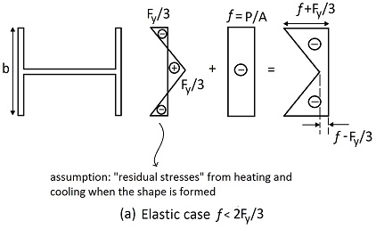
As we can see in the above figure (Fig (a)), the heating and cooling of the cross-section, which occur during the hot rolling process, has a very significant impact on the stress distribution that exists within the cross-section before and after the application of the service loads. The above figure shows the elastic case, which we can see is valid if our applied stress is less than approximately $\frac{2}{3}F_y$ . If this is true, then eq. 3 provides a good estimate of the critical stress, so long as the value of $\frac{x_0}{b}$ is taken as the fully elastic cross-section, namely, $\frac{x_0}{b}=.5$ (note that making this substitution reduces eq. 3 to eq. 2).

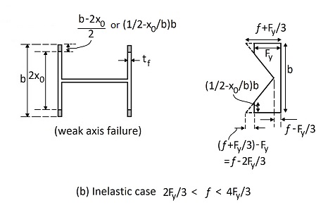
The above figure (Fig. (b)) shows the stress distribution in the cross-section if an applied load greater than $\frac{2}{3}F_y$ is applied. It should be noted that the applied stress, $f$ , is not the same as the average stress depicted in Fig. (b). Due to the “prestressing” effect of the residual stresses, it turns out that the average stress in Fig. (b) is less than the applied stress, $f$ . We will conservatively take the average stress in Fig. (b) to be equal to $F_{cr}$ , rather than $f$ .

Let’s find the compression force, $P_{cr}$ , from Fig. (b).

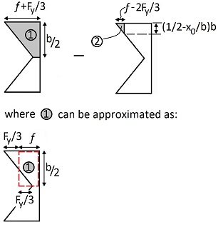
Observing the above figure, we can calculate $P_{cr}$ , as follows:

(4) $\begin{equation*} P_{cr}=4*\bigg[\underbrace{f}_{\text{ave stress over "1"}}*\frac{1}{2}bt_f-\underbrace{\frac{1}{2}(f-\frac{2}{3}F_y)}_{\text{ave stress over "2"}}(\frac{1}{2}-\frac{x_0}{b})bt_f\bigg] \end{equation*}$

Now, we’d like to eliminate the variable $f$ , which we introduced, and which we decided is not equal to $F_{cr}$ . So, we need an additional equation to eliminate it. This equation comes from similar triangles, as depicted below.

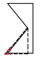
Using the above figure, which depicts two similar triangles, we can write the following expression:

$\begin{equation*} \frac{f-\frac{2}{3}F_y}{(\frac{1}{2}-\frac{x_0}{b})b}=\frac{\frac{2}{3}F_y}{\frac{b}{2}} \end{equation*}$

(5) $\begin{equation*} \rightarrow f=\bigg[1-\frac{x_0}{b}\bigg]\frac{4}{3}F_y \end{equation*}$

Eq. 5 $\rightarrow$ eq. 4 and $A \approx 2bt_f$ to eliminate $t_f$ , we get the following:

$\begin{equation*} P_{cr}=A F_y \bigg[1-\frac{4}{3}(\frac{x_0}{b})^2\bigg] \end{equation*}$

(6) $\begin{equation*} F_{cr}=F_y \bigg[1-\frac{4}{3}(\frac{x_0}{b})^2\bigg] \end{equation*}$

Recall that we had two unknowns, $F_{cr}$ and $\frac{x_0}{b}$ , and we needed two equations.
Our objective, of course, is to write the governing equations for weak axis elastic buckling of a wide flange I-shape.
Eq. 3 was our buckling equation that resulted from our Euler Buckling differential equation and our assumption about the tangent modulus, $E_t$ .
Eq. 6 is our equation that involves the shape’s residual stresses, the material yield stress, and a conservative approximation of $F_{cr}$ from Fig. (b).
We now have two equations (Eq. 3 and eq. 6) and two unknowns ( $F_{cr}$ and $\frac{x_0}{b}$ ).

Let’s vary $\frac{KL}{r}$ (a value that is known for a given column) and investigate how $\frac{x_0}{b}$ and $F_{cr}$ change. These results are shown in the table below.

The rightmost column of the above table are values of $F_{cr}$ obtained from the building code equations. These building code equations for $F_{cr}$ , which are empirical, are as follows:

Define a new parameter, called $\lambda_c$ , to be:

$\begin{equation*} \lambda_c=\frac{KL}{r}\sqrt{\frac{F_y}{\pi^2 E}} \end{equation*}$

For $\lambda_c < 1.5$ ,

$\begin{equation*} F_{cr}=.658^{\lambda_c^2}*F_y \end{equation*}$

For $\lambda_c >1.5$ ,

$\begin{equation*} F_{cr}=\frac{.877}{\lambda_c^2}*F_y \end{equation*}$

These building code equations for $F_{cr}$ apply to I-shapes, angles, channels, and tubes.

C. G. Salmon and J. E. Johnson, Steel Structures: Design and Behavior, 5th ed., New York, NY: Prentice Hall, 2008.
[Bibtex]

@BOOK{Salmon,
    Address        = {New York, NY},
    Author         = {Charles G. Salmon and John E. Johnson},
    Edition        = {5th},
    Publisher      = {Prentice Hall},
    Title          = {Steel Structures: Design and Behavior},
    Year           = {2008}
}

Leave a Reply Cancel reply