“Mechanics of Materials” is typically an engineering student’s first exposure to the important concepts relating to material properties, such as material strength and material stiffness. Material strength and stiffness are important for the analysis of structures, since the equations of static equilibrium are not enough to determine the distribution of forces within a complex structure. In addition, knowledge of material strength and stiffness is vital for the design of structures, where the size (and corresponding cost) of a component of a structure, such as a beam, depends on both its resistance to excessive deformation (primarily a function of stiffness), and its ability to resist damage (primarily a function of strength).

As we will see, beginning with this outline, two of the most important quantities in structural engineering are stress and strain. The stress and strain of a material are often linearly-related – a discovery that dates back to 1678, when Hooke famously stated “ut tensio, sic vis,” meaning, “as the extension, so the force.” The larger this ratio, the more stiff the material, and the greater its resistance to deformation. Keeping deformations small is sometimes a constraint in the design of structures.

A constraint that is even more often present in engineering design is to ensure that the material strength, which has units of stress, is not exceeded. Stress demands, unlike strains, are not so easy to “see” or directly measure, but stress is a quantity that engineers like to use for the purpose of comparing to material strength. Designing a structure so that the stress demands in all of its structural components remain less than their corresponding material strength values is one way that an engineer can ensure that the structure is safe to perform its intended function.

Hooke’s Law

$\mbox{Normal stress} = \frac{\mbox{force}}{\mbox{cross sectional area}} = \frac{\mbox{P}}{\mbox{A}} = \sigma$

(stress distribution is in units of $\frac{lb}{in^2}$ , psi, or $\frac{kip}{in^2}$ or $\frac{N}{m^2}$ , Pascal)

$\begin{equation*} \mbox{Normal strain} = \frac{\mbox{elongation}}{\mbox{length}} = \frac{\delta}{\mbox{L}} = \epsilon \mbox{ (fraction of change in length) } \end{equation*}$

Note: Strain is unitless!
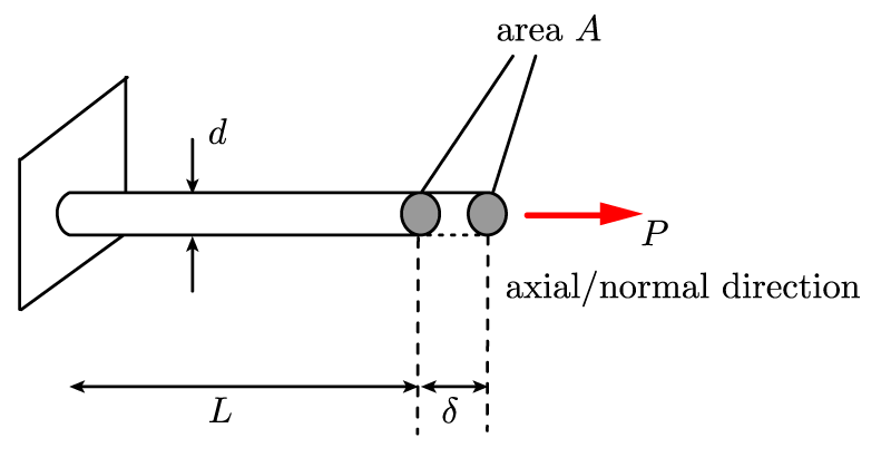
Note: As the rod elongates, the area shrinks $\longrightarrow$ the actual stress is slightly large than that assumed above. Similarly, the actual strain is actually $\frac{\delta}{L + \delta}$ , which is slightly smaller than that assumed above.
The most general form of Hooke’s Law is:

$\begin{equation*} \sigma=E*\epsilon \end{equation*}$

where $E$ = the modulus of elasticity (a material property)

Note: Unless stated otherwise, $P$ is assumed to be an equivalent force through the centroid of $A$ .

Note: As a practical rule $\sigma = \frac{P}{A}$ may be used with good accuracy at any point within a bar that is at least as far away from the force concentration as the lateral dimension of that bar ( $d$ or greater in the picture below).

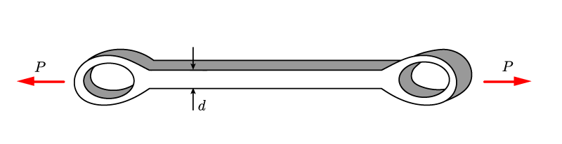
For non-uniform bars, such as the eyebar above, as long as you can make sure that failure will occur in the prismatic portion of the beam, it can be analyzed using the normal stress and strain equations above.

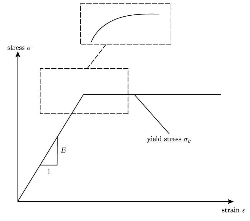
The above picture is a graph of stress versus strain for typical structural steel. We can see that the slope of the curve is $E$ , as one would expect according to the Hooke’s Law equation stated above. Many materials obey this linear relationship. In addition, this portion is called the “elastic” portion, because any structure that is stressed within the elastic portion will return to its original state upon release of stress.

The “yield stress” as shown on the graph is typically considered the limit of the material. Once the material reaches this stress, it continues to stretch or compress without any further load, and upon release of all load, will only partially return to its original state. This phenomenon is called “yielding.” The yield stress value, which is a material property, is typically considered the strength of the material. Grade 50 steel, for example, has a yield stress of 50 ksi.

Often materials are idealized as perfectly “elasto-plastic.” As we can see on the diagram above, the steel is perfectly elastic, then perfectly plastic (yielding portion = “plastic” portion). The dotted box in the diagram, which shows the more a smooth transition, is sometimes neglected.

In this topic, all materials will be assumed linear elastic!

$\begin{align*} \delta = \frac{PL}{AE} \qquad \text{ AE} &= \text{"axial rigidity"} \\ \delta = fP \qquad f &= \text{flexibility} = \frac{L}{AE} \left(\frac{\text{length change produced}}{\text{unit force}}\right) \\ P = k\delta \qquad k&= \text{stiffness} = \frac{AE}{L} \left(\frac{\text{force required}}{\text{unit of length change}}\right)^{*}\end{equation} \end{align*}$

* Note: this is the commonly written version of Hooke’s Law.

Sample Problem using Hooke’s Law

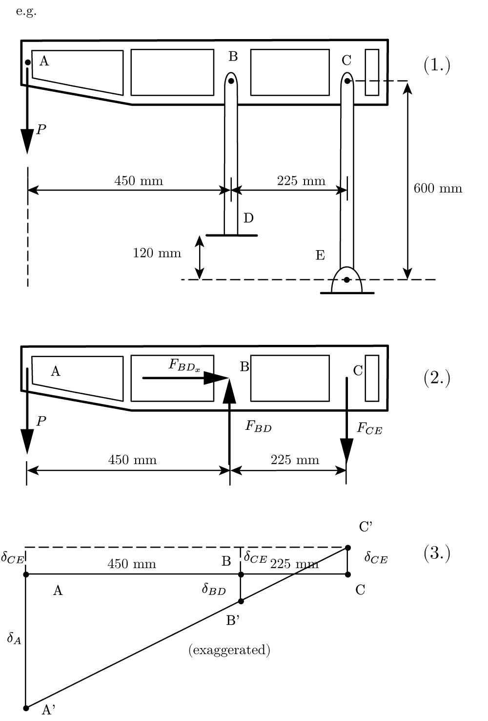
Given: Dimensions of frame shown below. $L_{BD}=480mm$ , $L_{CE}=600mm$ , $A_{BD}=1020mm^2$ , $A_{CE}=520mm^2$ , $E_{steel}=205GPa$
Find: Assuming member ABC to be rigid, find $P_{max}$ if the displacement at point A is limited to 1.0mm.

$\begin{align*} +\circlearrowleft\Sum M_B &: P(450) - F_{CE}(225) = 0 \Rightarrow F_{CE} = 2P \\ +\uparrow\Sum F_y &: F_{BD} - 2P - P = 0 \Rightarrow F_{BD} = 3P \\ +\rightarrow\Sum F_x &= 0 \Rightarrow F_{BDx} = 0 \\ \end{align*}$

$\begin{align*} \delta_{BD} &= \frac{(3P)(480*10^{-3})}{(205*10^9)(1020*10^{-6})} = 6.887P*10^{-9} m \text{ (shortening)}\\ \delta_{CE} &= \frac{(2P)(600*10^{-3})}{(205*10^9)(520*10^{-6})}=1.126P*10^{-8} m \text{ (lengthening)}\\ \end{align*}$

$\mathbf{B}$ moves to $\mathbf{B'}$ , $\mathbf{C}$ moves to $\mathbf{C'}$ , and $\mathbf{A}$ moves to $\mathbf{A'}$ by an amount $\delta_A$ .
From similar triangles (3.),

$\begin{align*} \frac{\delta_A + \delta_{CE}}{450 + 225} &= \frac{\delta_{BD} + \delta_{CE}}{225} \\ \frac{\delta_A + \delta_{CE}}{450 + 225} &= \frac{(\delta_A)_{\text{allowed}} + (1.126P_{max}*10^{-5} mm)}{450 mm + 225 mm} \\ \frac{\delta_{BD} + \delta_{CE}}{225} &= \frac{(6.887P_{max}*10^-6) + (1.126P_{max}*10^-5)mm}{225 mm} \\ \end{align*}$

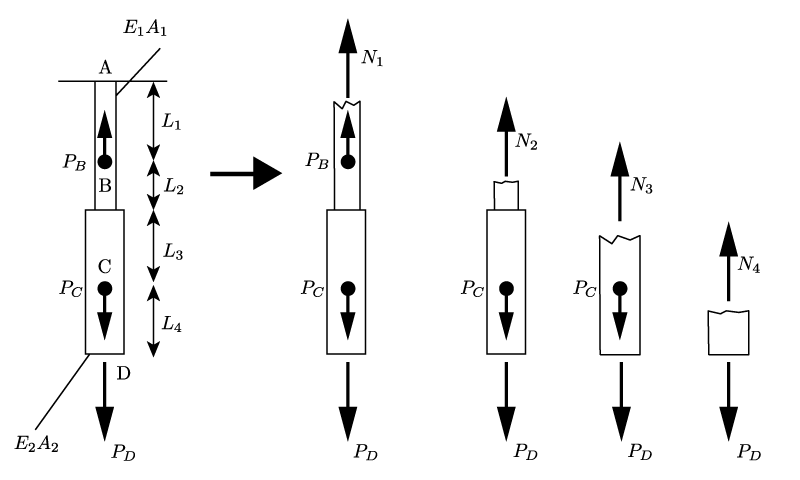
substitute $(\delta_A)_{\text{allowed}} = 1.0 mm$ , solve for $P_{max} \Rightarrow $P_{max} = \mathbf{23,200 N}$

Deformation of Axially Loaded Bar with Multiple Loads

Given: Bar made of multiple materials/cross sections with several axial loads.
Find: Deformation at point $\mathbf{D}$

$\begin{align*} +\uparrow \sum F_y&: N_1 + P_B - P_C - P_D = 0 \\ \Rightarrow N_1 &= P_C + P_D - P_B \\ N_2 &= N_3 = P_C + P_D \\ N_4 &= P_D \\ \delta_1 &= \frac{N_1 L_1}{E_1 A_1} \qquad \delta_2 = \frac{N_2 L_2}{E_1 A_1} \qquad \delta_3 = \frac{N_3 L_3}{E_2 A_2} \qquad \delta_4 = \frac{N_4 L_4}{E_2 A_2} \\ \delta_{total} &= \sum \delta \end{align*}$

Deformation of Tapered Bars in Tension Examples

For continuously varying loads or dimensions, the following integral applies:

$\begin{equation*} d\delta = \frac{N(x)dx}{EA(x)} \qquad \delta = \int_0^L \frac{N(x)}{EA(x)}dx \end{equation*}$

Given: Square beam loaded by its own weight with a density $(\rho = 10 kip/ft)$ , Young’s Modulus $(E = 2000ksi)$
Find: $\delta$ under the given load.

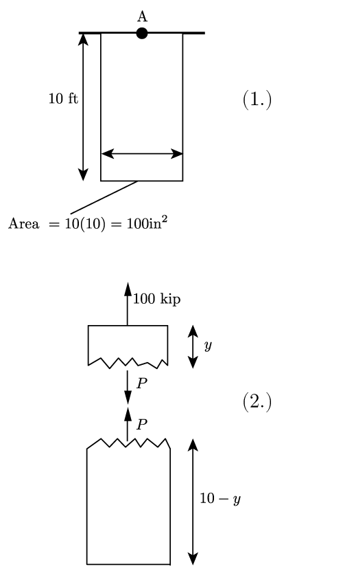
$\begin{align*} \text{Support reaction}&: \\ F_A &= \left(10 \frac{kip}{ft}\right)(10 ft) = 100 kip\\ \text{Top piece}&: \\ +\uparrow \sum F_y&: 100 - \left(10\frac{kip}{ft}\right)(y) - P = 0 \Rightarrow P = 100 - 10y\\ \text{Bottom piece}&: \\ +\uparrow \sum F_y &: P - \left(10 \frac{kip}{ft}\right)(10 - y) = 0 \Rightarrow P = 100 - 10y \\ \delta &= \int_0^10\frac{100 - 10y}{(100 in^2)(2000ksi)}dy = \frac{500 kip*ft}{200,000kip} = \mathbf{0.0025ft} \end{align*}$

Note: The general formula for length change of a bar (with constant area $A$ ) subjected to uniform $\frac{\text{force}}{\text{unit length}}$ is $\delta = \frac{PL}{2EA}$ ( $P = 100kips$ in above problem)

Given: Rectangular tapered beam of depth 10 in. loaded by its own weight. Same density and Young’s modulus material as the above problem.
Find: $\delta$

$\begin{align*} \text{Density: } \rho &= 10 \frac{kip}{ft} \left(\frac{1 ft}{(12 in)(100 in^2)}\right) = \frac{1kip}{120in^3} \\ \text{Support reaction}&:\\ F_A &= \left(\frac{120 + 80}{2}in^2\right)(10ft)\left(\frac{12in}{1ft}\right)\left(\frac{1 kip}{120 in^3}\right) = 100 kip \end{align*}$

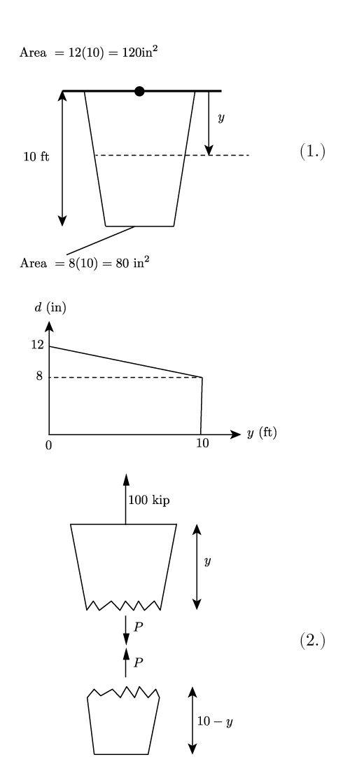
Note: This used the fact that for a linearly changing area $\Rightarrow$ Volume = (average area)(length).

$\begin{align*} A(y) &= d(y)*depth=\left(\frac{12-8}{0 - 10}y + 12\right)(10) = 120-4y\\ \text{Top piece} &:\\ + \uparrow \sum F_y &:100 - P - \left(\frac{120 + 120 - 4y)}{2}in^2\right)(y ft)*\left(\frac{12 in}{1 ft}\right)\left(\frac{1 kip}{120 in^3}\right) = 0 \\ \Rightarrow P &= \frac{1}{5}(y^2 - 60y + 500) \\ \delta &= \int_0^10 \frac{\frac{1}{5}(y^2 - 60y + 500)}{(120-4y)(2000)}dy = \mathbf{0.0022 ft} \end{align*}$

Note: The tapered bar has slightly less elongation than a prismatic bar of equal length and volume!
Note: The area must be constant or vary linearly or the problem is much more complex. For example, if the top length of the tapered bar is 12 in and the bottom length is 8 in, and it is a circular cylinder. So, $A=36*\pi$ and $16\pi$ respectively.

$\begin{equation*} A(y) = \frac{\pi}{4}[d(y)]^2 = \frac{\pi}{4}\left(\frac{12- 8}{0 - 10}y + 12 \right)^2 \end{equation*}$

$A(y)$ is NOT linear. So, finding needed volumes to determine the centroid is more complicated.