2nd Order Tensor Transformations

We already know:

(1) $\begin{equation*} \mathbf{a}=a_i\mathbf{e_i} \end{equation*}$

Similarly, we need to be able to express a higher order matrix, using tensor notation:

(2) $\begin{equation*} \mathbf{A}=A_{ij}\mathbf{e_ie_j} \end{equation*}$

$\mathbf{e_ie_j}$ is sometimes written: $\mathbf{e_i\otimes{e_j}}$ , where “ $\otimes$ ” denotes the “dyadic” or “tensor” product

e.x. $\mathbf{e_1\otimes{e_2}}= \begin{bmatrix}1\\0\\0\end{bmatrix} \begin{bmatrix}0 & 1 & 0\end{bmatrix}=\begin{bmatrix}0 & 1 & 0\\0 & 0 & 0\\0 & 0 & 0\end{bmatrix}$
As opposed to: $\mathbf{e_1 \cdot e_2}=\begin{bmatrix}1 & 0 & 0\end{bmatrix} \begin{bmatrix}0\\1\\0\end{bmatrix}=0$

$\mathbf{A}=$ sum of 3 x 3 matrices = 3 x 3 matrix

$\mathbf{A}=A_{ij}\mathbf{e_i\otimes{e_j}}=A_{11}\mathbf{e_1\otimes{e_1}}+A_{12}\mathbf{e_1\otimes{e_2}}+A_{13}\mathbf{e_1\otimes{e_3}}$
$+A_{21}\mathbf{e_2\otimes{e_1}}+A_{22}\mathbf{e_2\otimes{e_2}}+A_{23}\mathbf{e_2\otimes{e_3}}$
$+A_{31}\mathbf{e_3\otimes{e_1}}+A_{32}\mathbf{e_3\otimes{e_2}}+A_{33}\mathbf{e_3\otimes{e_3}}$

Recall eq. 3 in Section 1: Tensor Notation, which states that $x_i=A_{ij}b_j$ , where $\mathbf{A}$ is a 3×3 matrix, $\mathbf{b}$ is a vector, and $\mathbf{x}$ is the solution to the product between $\mathbf{A}$ and $\mathbf{b}$ . To see why this is so, we can consider the product between $\mathbf{A}$ and the basis vector $\mathbf{e_k}$ , and then consider the product between $\mathbf{A}$ and an arbitrary vector $\mathbf{b}$ . Before we do this, it should be mentioned that products between tensors and vectors (producing a vector) as well as products between two tensors (producing a tensor) will directly make use of the “dot product,” even though the “dot product” operator is sometimes thought of as a “scalar product.” The “dot product” treatment used consistently throughout this text, although mathematically a bit “sloppy,” enables one to use index notation to derive quantities in a very direct manner.

The “dot product” will be used in this text to signify the tensor product between a tensor and a vector or the tensor product between two tensors. This is consistent with most of the literature in solid mechanics. A small minority of authors, however, consider this to be “sloppy” math and insist, instead, that the dot product between tensors produce a scalar value. This distinction is very important since tensor products, which produce tensors, are prevalent in solid mechanics and this text will heavily use the “dot” convention when deriving important identities and quantities. Authors that use a different convention would use a very different approach for derivation, in particular where index notation is used.

(3) $\begin{equation*} \mathbf{A \cdot e_k} = A_{ij}\mathbf{e_i \otimes{e_j} \cdot e_k} = A_{ij}\mathbf{e_i}\delta_{jk}=(A_{ij}\delta_{jk})\mathbf{e_i}=A_{ik}\mathbf{e_i} \end{equation*}$

Note the use of the Kronecker delta in simplifying the expression in eq. 3.

Similarly,

(4) $\begin{equation*} \mathbf{A} \cdot \mathbf{b}=A_{ij}\mathbf{e_i}\mathbf{e_j} \cdot b_k\mathbf{e_k}=A_{ij}\mathbf{e_i}b_k\delta_{jk}=A_{ik}b_k\mathbf{e_i} \text{ or }\mathbf{A} \cdot \mathbf{b}=A_{ij}b_j\mathbf{e_i} \end{equation*}$

Again, the solution is a vector; this time with components $x_i=A_{ij}b_j$ , as expected (eq. 3 in Section 1: Tensor Notation).

note: Eq. 4 is standard matrix multiplication. We had to use a “dot” product to get the tensor algebra to work as a typical matrix – vector multiplication (we’ll see later that $\mathbf{A} \cdot \mathbf{B}$ also results in the standard matrix – matrix product). This is consistent with most of the literature in solid mechanics.

note: Remember, in the above derivations, only if $j=k$ is $\delta_{jk}$ non-zero. This was explained in eq. 2 in Section 1: Kronecker Delta. Note how this simplified the derivations. This is very common in tensor algebra.

So, consider eq. 3. Let’s “pick out” a particular component of this tensor, as follows:

Multiplying both sides by $\mathbf{e_j}\longrightarrow \mathbf{e_j \cdot A \cdot e_k=e_j} \cdot A_{ik}\mathbf{e_i}=\delta_{ij}A_{ik}=A_{jk}$
$\therefore$
$A_{jk}=\mathbf{e_j \cdot A \cdot e_k}$
or, re-written:

(5) $\begin{equation*} A_{ij}=\mathbf{e_i \cdot A \cdot e_j} \end{equation*}$

note: The LHS of eq. 5 is only one term. I.e. this is how you pick out a single term of a matrix.

note: For $1^{st}$ order: $a_i=\mathbf{a \cdot e_i}$ , where $a_i$ gives the component of $\mathbf{a}$ in the “ $i$ ” direction.

Consider the following coordinate system (see Figure):

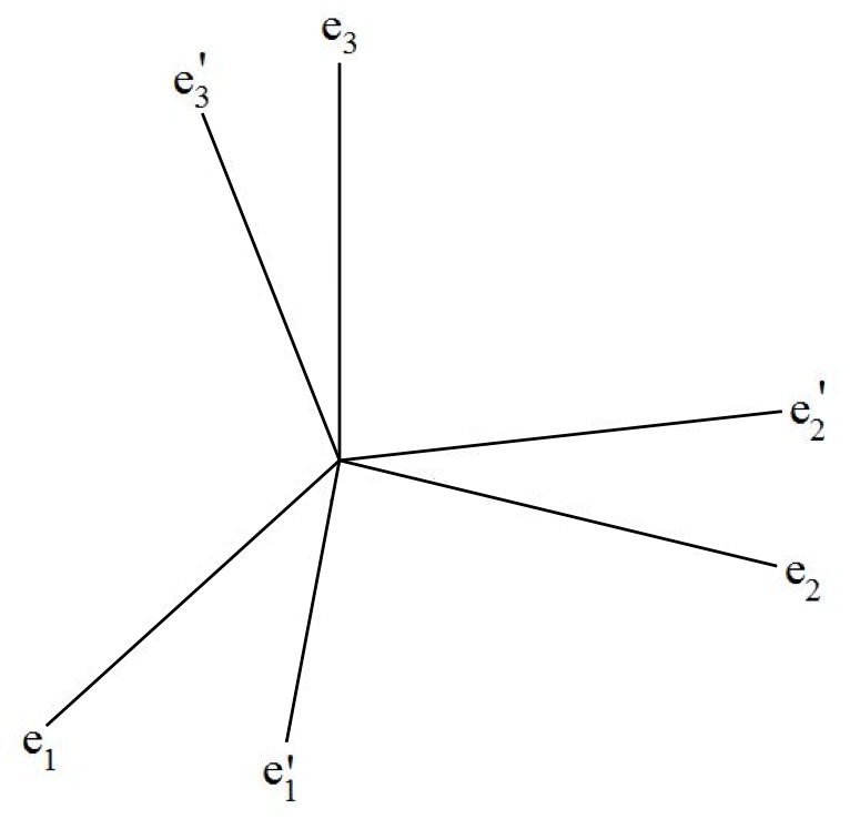
$\mathbf{e_{i}^{'}=Q \cdot e_i}$ ; $\mathbf{Q}=\text{rotation matrix }=Q_{mn}\mathbf{e_m \otimes e_n}$

we know: $\mathbf{e_{i}^{'}}=Q_{mn}\mathbf{e_m} \otimes \underbrace{\mathbf{e_n \cdot e_i}}_{\delta_{in}}=Q_{mi}\mathbf{e_m} \longrightarrow \mathbf{e_{i}^{'}} \cdot \mathbf{e_n}=Q_{mi}\underbrace{\mathbf{e_m \cdot e_n}}_{\delta_{mn}}=Q_{ni}$

$\longrightarrow Q_{ni}=\mathbf{e_{i}^{'} \cdot e_n}$ (terms [components] of a rotation matrix)

To be more useful, we need to show that $a_j=Q_{ji}a_{i}^{'}$ .

By definition, $\mathbf{a}=a_i\mathbf{e_i}=a_{i}^{'}\mathbf{e_{i}^{'}}$

Multiply both sides by $\mathbf{e_j}$ : $a_i \underbrace{\mathbf{e_i \cdot e_j}}_{\delta_{ij}}=a_{i}^{'}\underbrace{\mathbf{e_{i}^{'} \cdot e_j}}_{Q_{ji}}$

And, since $Q_{ji}=\mathbf{e_j \cdot e_{i}^{'}}=\mathbf{e_{i}^{'} \cdot e_j}$ (this should be obvious):

(6) $\begin{equation*} a_j=Q_{ji}a_{i}^{'} \end{equation*}$

note: $\mathbf{Q \cdot Q^{-1}}=\mathbf{Q^{-1} \cdot Q}=\mathbf{I}$ (this is true of any tensor)

$\mathbf{Q}$ is an “orthogonal” tensor. A particular identity of an orthogonal tensor can be written as follows:

(7) $\begin{equation*} (\mathbf{Q}\cdot\mathbf{u})\cdot(\mathbf{Q}\cdot\mathbf{v})=\mathbf{u\cdot v} \end{equation*}$

For an orthogonal tensor, $\mathbf{Q}$ (obeys eq. 7), it can be shown that $\mathbf{Q}^{T}=\mathbf{Q}^{-1}$ (pf can be found in [Asaro])

$\therefore$

$\mathbf{Q} \cdot \mathbf{Q}^{T}=\mathbf{Q}^{T} \cdot \mathbf{Q}=\mathbf{I}$

where $\mathbf{I}=\delta_{ij}\mathbf{e_i \otimes e_j}$
$=\mathbf{e_ie_i}=\mathbf{e_1e_1+e_2e_2+e_3e_3}$
$=\begin{bmatrix}1 & 0 & 0\\ 0 & 0 & 0\\ 0 & 0 & 0\end{bmatrix}+\begin{bmatrix}0 & 0 & 0 \\ 0 & 1 & 0 \\ 0 & 0 & 0\end{bmatrix}+\begin{bmatrix}0 & 0 & 0\\0 & 0 & 0\\ 0 & 0 & 1\end{bmatrix}$

From eq. 6, we know that $\mathbf{a}=\mathbf{Q \cdot a^{'}}$
$\mathbf{Q}^{T} \cdot \mathbf{a}=\underbrace{\mathbf{Q}^{T} \cdot \mathbf{Q}}_{\mathbf{I}} \cdot \mathbf{a}^{'}$
$\mathbf{a}^{'}=\mathbf{Q}^{T} \cdot \mathbf{a}$
$a_{i}^{'}=(Q^{T})_{ij} a_j$

(8) $\begin{equation*} a_{i}^{'}=Q_{ji} a_j \end{equation*}$

In eq. 8, $Q_{ji}=\mathbf{e_j \cdot e_{i}^{'}}$
(assuming we know the unit vectors defining the original and rotated coordinate systems).

What about transforming a tensor?
$\mathbf{A}=A_{ij}\mathbf{e_i \otimes e_j}$
$\mathbf{A}=A_{ij}^{'}\mathbf{e_{i}^{'} \otimes e_{j}^{'}}$
$\underbrace{\mathbf{e_{k}^{'} \cdot A \cdot e_{l}^{'}}}_{A_{kl}^{'}}=A_{ij}(\underbrace{\mathbf{\phantom{\sum}e_{k}^{'} \cdot e_i\phantom{\sum}}}_{Q_{ik}})(\underbrace{\mathbf{\phantom{\sum}e_j \cdot e_{l}^{'}\phantom{\sum}}}_{Q_{jl}})$

The following will be simply stated, and then proved:

(9) $\begin{equation*} A_{kl}^{'}=A_{ij}Q_{ik}Q_{jl}=Q_{ik}A_{ij}Q_{jl} \longrightarrow \mathbf{A'}=\mathbf{Q}^{T} \cdot \mathbf{A \cdot Q} \end{equation*}$

Tensor product practice and quick proof of eq. 9:

$\mathbf{A \cdot Q}=A_{ij}\mathbf{e_ie_j} \cdot Q_{kl}\mathbf{e_ke_l}=A_{ij}Q_{kl}\delta_{jk}\mathbf{e_i}\mathbf{e_l}=A_{ij}Q_{jl}\mathbf{e_ie_l}$

Now taking $\mathbf{Q}$ to be $\mathbf{Q}=Q_{tk}\mathbf{e_te_k}$ , we find:

$\mathbf{Q}^{T}\cdot(\mathbf{A}\cdot\mathbf{Q})=Q_{tk}\mathbf{e_ke_t}\cdot A_{ij}Q_{jl}\mathbf{e_ie_l}$

Thus, $\mathbf{Q}^{T}\cdot\mathbf{A}\cdot\mathbf{Q}=Q_{tk}A_{ij}Q_{jl}\delta_{ti}\mathbf{e_ke_l}=Q_{ik}A_{ij}Q_{jl}\mathbf{e_ke_l}$

Setting $\mathbf{A'}=\mathbf{Q}^{T}\cdot\mathbf{A}\cdot\mathbf{Q}$ , we can see that the components are $A_{kl}'=Q_{ik}A_{ij}Q_{jl}$ – i.e. the desired result (eq. 9)

note: We put a “dot” to get the tensor algebra to work. It’s really just a standard matrix product. If ever a product is written $\mathbf{AB}$ or $\mathbf{Ab}$ , in this text, it is probably a typo! Most of the literature in solid mechanics uses the same notation as in this text. Some authors omit the “dot” (e.x. $\mathbf{A\cdot B}=\mathbf{AB}$ ) except when using index notation. Some authors take $\mathbf{A\cdot B}$ to be the scalar product, which is a completely different definition, as opposed to a difference merely in notation. Fortunately, authors that take $\mathbf{A\cdot B}$ to be the scalar product are a small minority in solid mechanics.

R. J. Asaro and V. A. Lubarda, Mechanics of Solids and Materials, Cambridge, UK: Cambridge University Press, 2006.
[Bibtex]

@BOOK{Asaro,
    Address        = {Cambridge, UK},
    Author         = {Robert J. Asaro and Vlado A. Lubarda},
    Edition        = {},
    Publisher      = {Cambridge University Press},
    Title          = {Mechanics of Solids and Materials},
    Year           = {2006}
}

Leave a Reply Cancel reply