Principal Stresses

Again, let’s start with $\mathbf{t_n}$ :

$\mathbf{t_n}=\mathbf{n} \cdot \boldsymbol{\sigma}$

$\sigma_{nn}=\mathbf{t_n \cdot n = n} \cdot \boldsymbol{\sigma} \cdot \mathbf{n}$

For what $\mathbf{n}$ is $\sigma_{nn}$ maximized?

Remember, $\mathbf{n \cdot n}=1$

“Lagrange multiplier”= $\phi = \sigma_{nn}-\lambda(\mathbf{n \cdot n}-1)$

In index notation, $\phi=n_i \sigma_{ij} n_j - \lambda(n_in_i-1)$

$\frac{\partial \phi}{\partial n_k}=0$ to find local optimums

$\underbrace{\frac{\partial n_i}{\partial n_k}}_{\delta_{ik}}(\sigma_{ij}n_j)+(n_i\sigma_{ij})\underbrace{\frac{\partial n_j}{\partial n_k}}_{\delta_{jk}}-\lambda\underbrace{\frac{\partial n_i}{\partial n_k}}_{\delta_{ik}}n_i-\lambda\underbrace{\frac{\partial n_i}{\partial n_k}}_{\delta_{ik}}n_i=0$

Simplifying, we get: $\underbrace{\sigma_{kj}n_j}_{\text{or }\sigma_{ki}n_i} +n_i\sigma_{ik}-2\lambda n_k=0$ $\longrightarrow 2\sigma_{ik}n_i-2\lambda n_k=0$

This further reduces to: $\underbrace{\sigma_{ik}n_i}_{t_k}-\lambda n_k=0$ ; $t_k-\lambda n_k=0 \longrightarrow t_k=\lambda n_k$

$(\boldsymbol{\sigma}-\lambda \mathbf{I})\cdot \mathbf{n}=0 \longrightarrow$ Eigenvalue problem $\longrightarrow \lambda$ is precisely $\sigma_{\text{max, min}}$

This “Eigenvalue problem” was mentioned in Section 1: Trace, Scalar Product, Eigenvalues. An alternative proof of the principal stress eigenvalue problem can be found in [Boresi].

And, at the principal plane, traction is in the direction of the normal –i.e. no shear. (max shear = $\frac{\sigma_{\text{max}}-\sigma_{\text{min}}}{2}$ )

Principal shear stresses can be found in [Holzapfel].

Simple 2D e.x.: Problems like the following are typical in undergrad “mechanics of materials”, where Mohr’s Circle would be used to find the maximum stresses. Tensor methods are faster and can be more easily extended to 3D.

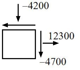
$\boldsymbol{\sigma}=\begin{bmatrix}-4200 & -4700 & 0\\-4700 & 12300 & 0 \\ 0 & 0 & 0\end{bmatrix} \longrightarrow \lambda_1 = -5445$ ; $\lambda_2=13540$

Principal direction, $\mathbf{n}_{\lambda_1}=\begin{bmatrix}-.97\\-.26\\0\end{bmatrix}$
$\theta_p = tan^{-1}\frac{.26}{.97}=75^\text{o}$

The above values of stress and angle agree with the transformation equations from undergrad, of course.

G. A. Holzapfel, Nonlinear Solid Mechanics: A Continuum Approach for Engineering, Baffins Lane, Chichester, West Sussex PO19 1UD, England: John Wiley & Sons Ltd., 2000.
[Bibtex]

@book{holzapfel,

    address = {Baffins Lane, Chichester, West Sussex PO19 1UD, England},

    author = {Holzapfel, Gerhard A.},
    publisher = {John Wiley \& Sons Ltd.},

    title = {{Nonlinear Solid Mechanics: A Continuum Approach for Engineering}},

    year = {2000}
}

A. P. Boresi, R. J. Schmidt, and O. M. Sidebottom, Advanced mechanics of materials, Wiley New York, 1993, vol. 5.
[Bibtex]

@book{Boresi,
  title={Advanced mechanics of materials},
  author={Boresi, Arthur Peter and Schmidt, Richard Joseph and Sidebottom, Omar M},
  volume={5},
  year={1993},
  publisher={Wiley New York}
}

Leave a Reply Cancel reply