Strain Tensors

Recall from eq. 1 in Section 2: Strain, that $\mathbf{dx=F \cdot dX}$

Since $\mathbf{dx=(I+u\nabla) \cdot dX}$ , $\mathbf{F=I+u\nabla}$
or, in index notation:

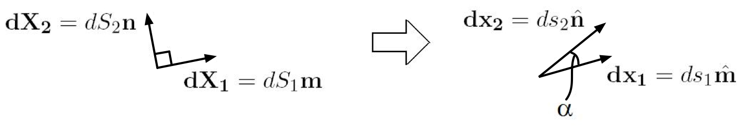
$F_{ij}=\delta_{ij}+\frac{\partial u_i}{\partial X_j}=\frac{\partial x_i}{\partial X_j}$ , since $\mathbf{du=[(x+dx)-(X+dX)]-(x-X)=dx-dX}$
and $\frac{\partial X_i}{\partial X_j}=\delta_{ij}$ , by definition.

The tensor, $\mathbf{F}$ , is typically referred to as the “deformation gradient.” To see how $\mathbf{F}$ is found in 2D and 3D in an actual FEA application, see Finite Element Coordinate Mapping [McGinty].

In matrix form:

(1) $\begin{equation*} \mathbf{u \nabla}=\begin{bmatrix}\frac{\partial u_1}{\partial X_1} & \frac{\partial u_1}{\partial X_2} & \frac{\partial u_1}{\partial X_3}\\ \frac{\partial u_2}{\partial X_1} & \frac{\partial u_2}{\partial X_2} & \frac{\partial u_2}{\partial X_3}\\ \frac{\partial u_3}{\partial X_1} & \frac{\partial u_3}{\partial X_2} & \frac{\partial u_3}{\partial X_3} \end{bmatrix} \end{equation*}$

$\mathbf{F}=\text{``deformation gradient''}$ :

(2) $\begin{equation*} \mathbf{F}=\begin{bmatrix}\frac{\partial x_1}{\partial X_1} & \frac{\partial x_1}{\partial X_2} & \frac{\partial x_1}{\partial X_3}\\ \frac{\partial x_2}{\partial X_1} & \frac{\partial x_2}{\partial X_2} & \frac{\partial x_2}{\partial X_3}\\ \frac{\partial x_3}{\partial X_1} & \frac{\partial x_3}{\partial X_2} & \frac{\partial x_3}{\partial X_3} \end{bmatrix} \end{equation*}$

$\mathbf{F}$ is sometimes called the “stretch” tensor

Now, consider how the length of any element or fiber within the continuum may change under deformation. To find such length “magnitudes” we can take dot products as follows:

$dS^2=\mathbf{dX \cdot dX}$ ( $dS$ = length $\mathbf{dX}$ )
$ds^2=\mathbf{dx \cdot dx}$ ( $ds$ = length $\mathbf{dx}$ )
$\mathbf{dx=F \cdot dX=dX \cdot F}^{T}$

note: you can’t do this transpose manipulation as easily if multiplying two tensors, but it works for two vectors or a vector and a tensor (use indices to easily prove)

$ds^2=\mathbf{dX} \cdot \mathbf{F}^{T} \cdot \mathbf{F} \cdot \mathbf{dX}$

note: $\mathbf{F}^{T} \cdot \mathbf{F} = \mathbf{C} =$ “Right C – G” (Cauchy – Green) deformation tensor. The reason for this name will become clear once we begin discussion our on “polar decomposition” theory.

(3) $\begin{equation*} \frac{ds^2-dS^2}{dS^2}=\frac{\mathbf{dX \cdot (F}^{T} \cdot \mathbf{F-I) \cdot dX}}{\mathbf{dX \cdot dX}}=2E_{nn} \end{equation*}$

where the Lagrangian Strain Tensor (or Green-Lagrange Strain Tensor) is: $\mathbf{E}=\frac{1}{2}(\mathbf{F}^{T} \cdot \mathbf{F-I})$

(4) $\begin{equation*} \mathbf{E}=\frac{1}{2}(\mathbf{C-I}) \end{equation*}$

$\mathbf{E \cdot n} =$ strain vector on a plane whose normal vector is $\mathbf{n}$ (the actual location in space is specified within $\mathbf{E}$ )
$E_{nn}=\mathbf{n \cdot E \cdot n}=$ strain (scalar) in direction $\mathbf{n}$

note:
From eq. 3, $E_{nn}=\frac{ds^2-dS^2}{2dS^2}=\frac{(ds-dS)(ds+dS)}{2dS^2}$
Suppose $ds=dS$ (infinitesimal deformation):
$E_{nn}=\frac{(ds-dS)(ds+dS)}{2dS^2} \approx \frac{(ds-dS)2dS}{2dS^2} = \frac{ds-dS}{dS}=\epsilon_{nn}$
i.e. $\epsilon=\frac{\Delta L}{L}$

what about $\mathbf{m \cdot E \cdot n}$ ?

e.x.
Suppose $\mathbf{n}$ and $\mathbf{m}$ are orthogonal in the undeformed configuration.
Since $\mathbf{E \cdot n}$ is the strain vector on a plane whose unit normal is $\mathbf{n}$ ,
$\mathbf{m \cdot E \cdot n}$ is the component of $\mathbf{E \cdot n}$ in direction $\mathbf{m}$ .
i.e. if $\mathbf{m}$ is in the plane of interest (orthogonal to $\mathbf{n}$ ), then $\mathbf{m \cdot E \cdot n}$ is the shear strain

We know that: $\mathbf{dx_1=F \cdot dX_1}$ ; $\mathbf{dx_2=F \cdot dX_2}$

So, $\mathbf{dx_1 \cdot dx_2 - dX_1 \cdot dX_2}=\mathbf{F}\cdot\mathbf{dX_1} \cdot \mathbf{F}\cdot \mathbf{dX_2}-\mathbf{dX_1 \cdot dX_2}$

From eq. 3 and recalling that $\mathbf{F} \cdot \mathbf{dX} = \mathbf{dX} \cdot \mathbf{F}^{T}$ , we get:
$\mathbf{dx_1 \cdot dx_2 - dX_1 \cdot dX_2}=2\mathbf{dX_1 \cdot E \cdot dX_2}$

$ds_1ds_2\underbrace{\hat{\mathbf{m}} \cdot \hat{\mathbf{n}}}_{cos\alpha}-0=2dS_1dS_2\underbrace{\mathbf{\hat{m}} \cdot \mathbf{E} \cdot \mathbf{\hat{n}}}_{E_{mn}}$ , where $\mathbf{\hat{m}}$ and $\mathbf{\hat{n}}$ are unit vectors

note: $\mathbf{dX_1\cdot dX_2}$ is “zero” on the LHS of the above equation because $\mathbf{\hat{m}}$ and $\mathbf{\hat{n}}$ are originally orthogonal
$E_{mn}=\frac{1}{2}\frac{ds_1}{dS_1}\frac{ds_2}{dS_2}cos\alpha$
where $\frac{ds_1}{dS_1}$ is the “stretch ratio”

note: As seen in the figure below, $\gamma = \frac{\pi}{2}-\alpha$ $\therefore cos\alpha = sin\gamma$

$E_{mn}=\frac{1}{2}\frac{ds_1}{dS_1}\frac{ds_2}{dS_2}sin\gamma$
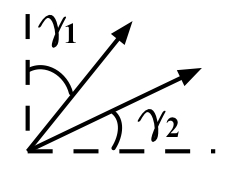
Infinitesimal engineering shear strain = $\epsilon_{xy}=\frac{1}{2}(\gamma_1+\gamma_2)=\frac{1}{2}\gamma$
Does our shear strain reduce to this value for infinitesimal deformation?

For infinitesimal deformation, $\frac{ds_1}{dS_1}=1$ ; $\frac{ds_2}{dS_2}=1$ ; $sin\gamma = \gamma$
$\longrightarrow E_{mn}=\frac{1}{2}(1)(1)(\gamma)=\frac{1}{2}\gamma$
$\longrightarrow E_{mn} \approx \epsilon_{mn}$ for linear infinitesimal deformation

We can also see from the following equation (eq. 5) that, in general, $\epsilon_{ij}=\frac{1}{2}(\frac{\partial u_i}{\partial X_j}+\frac{\partial u_j}{\partial X_i})$ for linear infinitesimal deformation (higher order terms are neglected).

For large (“finite”) strain:

(5) $\begin{equation*} E_{ij}=\frac{1}{2}\left(\frac{\partial u_i}{\partial X_j}+\frac{\partial u_j}{\partial X_i}+\frac{\partial u_k}{\partial X_i}\frac{\partial u_k}{\partial X_j}\right) \end{equation*}$

To prove, first consider: $F_{ij}=\delta_{ij}+\frac{\partial u_i}{\partial X_j}$ $\longrightarrow \mathbf{F=I+u\nabla}$

Now, from eq. 3, $\mathbf{E}=\frac{1}{2}(\mathbf{F}^{T} \cdot \mathbf{F-I})=\frac{1}{2}[(\mathbf{I+\nabla u}) \cdot (\mathbf{I+u\nabla})-\mathbf{I}]$
$=\frac{1}{2}[\mathbf{I+u\nabla+\nabla u+(\nabla u) \cdot (u\nabla)-I}]=\frac{1}{2}[\mathbf{u\nabla+\nabla u+(\nabla u) \cdot (u\nabla)}]$

Recall the definition of $\mathbf{\nabla u}$ from the figure at the beginning of this chapter, and recall that $\mathbf{u\nabla}$ is the transpose of $\mathbf{\nabla u}$

Eulerian strain:
Here, “Eulerian strain” is simply referring to a measure of strain that is defined in spatial coordinates. Under rigid body rotation, the Eulerian strain values will change, whereas the Lagrangian strain tensor is invariant to rigid body rotation. In other words, the coordinate system in which $\mathbf{E}$ is calculated (the “material” coordinate system) rotates with rigid body rotation. The coordinate system in which $\mathbf{e}$ is calculated (the “spatial” coordinate system) remains constant.

$\mathbf{dx=F \cdot dX} \longrightarrow \mathbf{dX=F}^{-1} \cdot \mathbf{dx}=\mathbf{dx} \cdot \mathbf{F}^{-T}$

Similar to the way that we derived $\mathbf{E}$ , let’s consider the difference in lengths of any particular element, or fiber, within our strain potato, before and after deformation.

$ds^2-dS^2=\mathbf{dx \cdot dx - dX \cdot dX=dx \cdot dx - dx \cdot F}^{-T} \cdot \mathbf{F}^{-1} \cdot \mathbf{dx}=\mathbf{dx} \cdot (\mathbf{I-F}^{-T} \cdot \mathbf{F}^{-1}) \cdot \mathbf{dx}$
$ds^2-dS^2=2\mathbf{dx} \cdot \mathbf{e} \cdot \mathbf{dx}$
where the Eulerian Strain Tensor (sometimes called the Almansi Strain Tensor) is: $\mathbf{e}=\frac{1}{2}(\mathbf{I-F}^{-T} \cdot \mathbf{F}^{-1})$

(6) $\begin{equation*} \mathbf{e}=\frac{1}{2}\left(\mathbf{I-B}^{-1}\right) \end{equation*}$

where $\mathbf{B}=$ Left C-G Tensor = $\mathbf{F \cdot F}^{T}$

$(\mathbf{B}^{-1}=\mathbf{F}^{-T} \cdot \mathbf{F}^{-1})$ , which is easy to prove using indices

$\mathbf{dX \cdot dX=dx \cdot}\underbrace{\mathbf{F}^{-T} \cdot \mathbf{F}^{-1}}_{\mathbf{B}^{-1}} \cdot \mathbf{dx}$
This is analogous to the previously derived $\mathbf{dx \cdot dx=dX \cdot F}^{T} \cdot \mathbf{F \cdot dX}$

Proof comes from:
$\mathbf{dX=F}^{-1} \cdot \mathbf{dx=dx \cdot F}^{-T}$

We’ll see the physical meaning of $\mathbf{B}$ and $\mathbf{C}$ when we discuss “polar decomposition.”

How is $\mathbf{e}$ related to $\mathbf{E}$ ?

$\mathbf{E}=\frac{1}{2}(\mathbf{F}^{T} \cdot \mathbf{F-I})$ ; $\mathbf{e}=\frac{1}{2}(\mathbf{I-F}^{-T} \cdot \mathbf{F}^{-1})$
$\mathbf{E=F}^{T} \cdot \underbrace{\frac{1}{2}(\mathbf{I-F}^{-T} \cdot \mathbf{F}^{-1})}_{\mathbf{e}} \cdot \mathbf{F}$
$\mathbf{e=F}^{-T} \cdot \underbrace{\frac{1}{2}(\mathbf{F}^{T} \cdot \mathbf{F-I})}_{\mathbf{E}} \cdot \mathbf{F}^{-1}$
$\mathbf{B}^{-1}=\mathbf{F}^{-T} \cdot \mathbf{F}^{-1} \longrightarrow B_{ij}^{-1}=F_{ik}^{-T} \cdot F_{kj}^{-1}$
(To convince yourself that these subscripts are correct, simply write out the matrix multiplication long-hand, summing only the dummy index “k”)

Since $\frac{\partial X_i}{\partial x_j}=\delta_{ij}-\frac{\partial u_i}{\partial x_j}=F_{ij}^{-1}$ ,
$B_{ij}^{-1}=(\delta_{ik}-\frac{\partial u_k}{\partial x_i})(\delta_{kj}-\frac{\partial u_k}{\partial x_j})=\delta_{ij}-\frac{\partial u_j}{\partial x_i}-\frac{\partial u_i}{\partial x_j}+\frac{\partial u_k}{\partial x_i}\frac{\partial u_k}{\partial x_j}$

(7) $\begin{equation*} \mathbf{e}=\frac{1}{2}(\mathbf{I-B}^{-1}) \longrightarrow e_{ij}=\frac{1}{2}(\delta_{ij}-B_{ij}^{-1})=\frac{1}{2}(\frac{\partial u_i}{\partial x_j}+\frac{\partial u_j}{\partial x_i}-\frac{\partial u_k}{\partial x_i}\frac{\partial u_k}{\partial x_j}) \end{equation*}$

If only infinitesimal deformation, and so long as no significant rigid body rotations are present, then $E_{ij} \approx e_{ij} \approx \epsilon_{ij}=\frac{1}{2}(\frac{\partial u_i}{\partial X_j}+\frac{\partial u_j}{\partial X_i})$
(this formula may be familiar from undergrad, for example)

Leave a Reply Cancel reply