Tabulated and Calibrated Models

In the past, experimental constants would typically be found by hand. Given a known material, it can be time-consuming to identify their parameters, even after the necessary experimental tests have been performed – e.g. since hyperelastic materials are nonlinear by definition, matching the experimental data is not so trivial as finding the slope of a uniaxial stress-strain curve, as would be the case for a linear material. The Mooney-Rivlin example in the last section (Section 6: Phenomenological and Micromechanical Models) showed that the procedure for obtaining experimental constants can be cumbersome. For more advanced hyperelastic models, finding the experimental constants would be even more difficult. More recently, two methods have been developed to “fit” a particular material to a particular hyperelastic model – the “tabulated” method and the “calibration” method.

Before we look at a particular tabulated model as well as a particular method for calibrating a model, consider that for many hyperelastic models, uniaxial data is sufficient to fully characterize their behavior. Exceptions would include models that are heavily influenced by higher order strain invariants. Regardless, uniaxial data is the most common kind of experimental data that is used for characterizing materials – hyperelastic materials included. In fact, both of the following examples will fit a hyperelastic model to uniaxial data, at the exclusion of any other kind of experiment data.

These characterization methods may be considered “curve-fitting” techniques, but keep in mind that the hyperelastic models that we are attempting to match to a uniaxial curve are tensorial, not scalar-valued. Using a tabulated approach, the challenge is to take a hyperelastic function, which forms a work-conjugate constitutive relationship that naturally extends to a 3D environment, and modify it to “grab” data from tabulated uniaxial stress-strain data. A particular tabulated approach developed by Stefan Kolling of Daimler AG, in collaboration with P.A. Du Bois of LSTC and David Benson of UCSD [Benson], will be presented, which is based on the Ogden model and generates a “perfect fit.”

(1) $\begin{equation*} f_0(\lambda_i)=\sum_{x=0}^\infty\lambda_i^{(-1/2)^x}\sigma_0\left(\lambda_i^{(-1/2)^x}-1\right) \end{equation*}$

(2) $\begin{equation*} \sigma_i=\frac{1}{III_\mathbf{V}}\left(f_0(\lambda_i)-\frac{1}{3}\sum_{n=1}^3f_0(\lambda_n)\right)+K\frac{III_\mathbf{V}-1}{III_\mathbf{V}} \end{equation*}$

The complete derivation of eq. 1 and eq. 2 can be found in Appendix C.4, based on the descriptions provided in [Benson].

In a simplified FEA algorithm (no rates/hypoelasticity), the series expressed above (eq. 1), which calculates a single value of $f_0(\lambda_i)$ from the uniaxial data by summing (over “ $x$ ”) to $\infty$ , would be terminated once a reasonable tolerance is met. In addition, a sufficient number of $f_0(\lambda_i)$ values could be calculated, where each value is calculated from eq. 1 and corresponds to a particular value of $\lambda_i$ . The number of $f_0(\lambda_i)$ values could perhaps be equal to the number of $\sigma_0(\epsilon_{0i})$ values that have been provided by the user, presumably from a uniaxial engineering stress vs. engineering strain plot. Note that all such $f_0(\lambda_i)$ values can be found during the initialization of the FEA problem, prior to the start of the simulation.

In solving actual problems using this material model (though this is still only for illustrative purposes, since real problems involve time and necessitate a hypoelastic constitutive formulation), the actual stretches are the eigenvalues of $\mathbf{V}$ and would be determined from the actual loading. $\sigma_1$ , $\sigma_2$ , $\sigma_3$ , which are the eigenvalues of the Cauchy stress, $\boldsymbol{\sigma}$ , can be calculated from eq. 2, where “ $i$ ” in eq. 2 refers to the eigenvalue $1$ , $2$ , or $3$ . Obtaining the Cauchy stress, $\boldsymbol{\sigma}$ , from its eigenvalues and eigenvectors involves just a single transformation.

While the original form of the Ogden model (eq. 7 in Section 6: Phenomenological and Micromechanical Models) contains an arbitrarily large number of constants, it is not necessarily true that the Ogden model, in its original form, can fit any uniaxial stress vs. strain curve. In its original form, the Ogden model contains the constants $\mu_s$ and $\alpha_s$ , and these constants (of which there exist $2m$ of them) would be solved simultaneously. One possible way to attempt this would be to start with eq. 1, where we recall that the left-hand-side of eq. 1 is $\sum_{s=1}^m\mu_s\lambda_i^{*\alpha_s}=f_0(\lambda_i)$ . It is not clear that creating multiple equations from eq. 1 and solving simultaneously for these constants is feasible.

The method presented, on the other hand, which is referred to as a “tabulated” method, can fit any uniaxial curve, perfectly. One can consider that this tabulated method is possible because of a number of particular characteristics in the original Ogden expression (eq. 7 in Section 6: Phenomenological and Micromechanical Models), and clever “tricks” employed by the authors of the tabulated model [Benson], which are shown in Appendix C.4.

The value of this “tabulated” method cannot be understated: it makes possible the exact fit to any uniaxial stress vs. strain experimental data. The material would then be characterized by Ogden hyperelasticity, which, in theory should work quite well for any type of loading condition that the material may see (torsion, bending, etc.). Viscoelasticity would be the primary concern, and this will be briefly discussed at the end of this chapter.

A “calibration” method will be shown next, and then the two methods will be briefly compared. The figure below is a screen-shot from a software called MCalibration, developed by Jorgen Bergstrom of Veryst Engineering $^{\text{\textregistered}}$ . MCalibration contains a library of materials called PolyUMod [Bergstrom]. Contained within this library are many hyperelastic materials, including all of the ones discussed in the previous section.

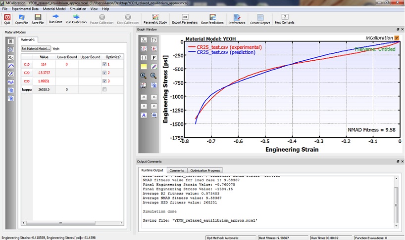
Data from a uniaxial compression experiment was loaded into MCalibration. We can assume, here, that the compression data represents the relaxed equilibrium response of the material – in other words, it is hyperelastic. The Yeoh model [Yeoh] was then calibrated, since this model provided a better fit, for this particular data set, compared to, for example, the Arruda-Boyce model. We can see that the fit is still not perfect. More information on the Yeoh model can be found in [Holzapfel] and [Bergstrom]. More information on the optimization algorithm that is used by MCalibration can be found in [Bergstrom]. It’s also interesting to note that the “rule-of-thumb” for the three constants in the Yeoh model (see previous section) give a result that is pretty close to the optimized values.

The advantage of the tabulated method, as stated previously, is that it will match any uniaxial curve, exactly, and take almost no computational effort to do so. A disadvantage of the tabulated method is that physical material properties never enter the conversation, so error in the uniaxial data can go unrecognized. Still, there are surprisingly very few tabulated models, like the one that has been presented, which are built from hyperelastic functions. This may be due to concerns related to the treatment of viscoelasticity, as will be briefly discussed.

Viscoelasticity

Perhaps the real reason that we don’t see more tabulated models is because for many kinds of polymers and for many applications that involve polymers, viscoelastic rate effects on loading and unloading behavior are as important as the underlying hyperelastic component of behavior. In reality, it is extremely difficult to obtain the relaxed equilibrium response of an elastomer, and so even a “quasi-static” uniaxial test will have different loading and unloading response. In other words, hyperelasticity is only one aspect of the response of an elastomer under realistic loading rates.

The specific implementation of the tabulated model previously described [Benson] is the LS-DYNA material model called:
$^{\ast}$ MAT_SIMPLIFIED_RUBBER_WITH_DAMAGE [Hallquist]

While this model can handle a user-defined uniaxial loading curve as well as an unloading curve, it does not handle hyper-viscoelasticity in a physical sense. This is why the developers of the model [Benson] use the word “simplified” and “damage” to describe the hysteretic behavior capability. No tabulated method, to the author’s knowledge, exists that can handle both hyperelasticity and viscoelasticity in a physical sense. The PolyUMod library, however, consists of many viscoelastic options, and MCalibration is capable of “fitting” uniaxial hysteretic data using models that contain components of both hyperelasticity and viscoelasticity. This topic, however, is beyond the scope of this text.

J. Bergstrom, PolyUMod User’s Manual, v.1.8.7 ed., Needham, MA: Veryst Engineering, LLC, 2009.
[Bibtex]

@BOOK{PolyuMod,
    Address        = {Needham, MA},
    Author         = {Jorgen Bergstrom},
    Edition        = {v.1.8.7},
    Publisher      = {Veryst Engineering, LLC},
    Title          = {PolyUMod User's Manual},
    Year           = {2009}
}

G. A. Holzapfel, Nonlinear Solid Mechanics: A Continuum Approach for Engineering, Baffins Lane, Chichester, West Sussex PO19 1UD, England: John Wiley & Sons Ltd., 2000.
[Bibtex]

@book{holzapfel,

    address = {Baffins Lane, Chichester, West Sussex PO19 1UD, England},

    author = {Holzapfel, Gerhard A.},
    publisher = {John Wiley \& Sons Ltd.},

    title = {{Nonlinear Solid Mechanics: A Continuum Approach for Engineering}},

    year = {2000}
}

J. Hallquist, LS-DYNA Keyword user�s manual, version 971, Livermore, CA: Livermore Software Technology, 2007.
[Bibtex]

@book{DYNA,

  title={LS-DYNA Keyword user�s manual, version 971},

  author={Hallquist, J.},

  url={},

  year={2007},

  publisher={Livermore Software Technology}
,
  Address= {Livermore, CA},}

S. Kolling, P. Bois, D. Benson, and W. Feng, “A tabulated formulation of hyperelasticity with rate effects and damage,” Computational Mechanics, vol. 40, pp. 885-899, 2007.
[Bibtex]

@article {Benson_two,
   author = {Kolling, S. and Bois, P. and Benson, D. and Feng, W.},
   affiliation = {DaimlerChrysler AG, EP/SPB HPC X271 71059 Sindelfingen Germany},
   title = {A tabulated formulation of hyperelasticity with rate effects and damage},
   journal = {Computational Mechanics},
   publisher = {Springer Berlin / Heidelberg},
   issn = {0178-7675},
   keyword = {Engineering},
   pages = {885-899},
   volume = {40},
   issue = {5},
   note = {10.1007/s00466-006-0150-x},
   year = {2007}
}

O. H. Yeoh, “Some forms of the strain energy function for rubber,” Rubber Chem. Technol., vol. 66, iss. 5, pp. 754-771, 1993.
[Bibtex]

@ARTICLE{Yeoh,
author={Yeoh, O.H.},
journal={Rubber Chem. Technol.},
title={Some forms of the strain energy function for rubber},
year={1993},
volume={66},
number={5},
pages={754 -771},
keywords={},
}

J. Bergstrom, Mechanics of Solid Polymers: Theory and Computational Modeling, William Andrew, 2015.
[Bibtex]

@book{Bergstrom_book,
  title={Mechanics of {S}olid {P}olymers: {T}heory and {C}omputational {M}odeling},
  author={Bergstrom, Jorgen},
  volume={},
  year={2015},
  publisher={William Andrew}
}

Leave a Reply Cancel reply