Phenomenological and Micromechanical Models

Hyperelastic constitutive models can be divided into two categories: phenomenological models and micro-mechanical models. Both phenomenological and micro-mechanical models can capture the behavior of a wide range of polymers. Whereas some polymers are compressible, and some polymers can strain elastically an order of magnitude more than others, polymers, generally-speaking, exhibit the same main characteristics, namely, highly nonlinear material behavior. Traditional phenomenological models are not derived from any underlying micro-mechanical physics, but are formed in a manner that seeks to minimize computational and experimental effort while capturing the overall behavior for a particular subset of polymers – e.g. elastomers that stiffen in compression and soften in tension. Four phenomenological models will be presented here: Mooney-Rivlin rubber [Mooney] [Rivlin], Yeoh rubber [Yeoh], Blatz-Ko foam [Blatz], and Ogden rubber [Ogden]. Micro-mechanical models, on the other hand, capture some of the underlying physical mechanisms of the materials. Micro-mechanical models have the most potential for improvement, and there are already some micro-mechanical models that can extend to unusual kinds of polymers, where traditional models would diverge from real behavior [Bergstrom and Boyce]. Here, only one micro-mechanical model will be presented: Arruda-Boyce rubber [Arruda]. The Arruda-Boyce model, in its original form [Arruda], can handle typical elastomers, but, like any hyperelastic model, will be unable to capture the hyperelastic behavior of all polymers.

Mooney-Rivlin e.x. 1

Consider a rectangular block under tensile stress in $X_1$ direction (simple extension test) that causes the stretch in that direction of amount $\lambda_1$ . If the material of the block is an incompressible “Mooney-Rivlin” rubber [Mooney] [Rivlin] with Strain Energy Density (sometimes called Helmholtz Free Energy):

(1) $\begin{equation*} \phi=\frac{1}{2}\mu \left[\left(\frac{1}{2}+\beta\right)(I_B-3)+\left(\frac{1}{2}-\beta\right)(II_B-3)\right] \end{equation*}$

where $\mu$ and $\beta$ are material constants, find the stress required to produce this deformation:

Incompressible $\rightarrow$ $\boldsymbol{\sigma}=-\rho_0\mathbf{I}+2\left[\left(\frac{\partial \phi}{\partial I_B}\right)\mathbf{B}-\left(\frac{\partial \phi}{\partial II_B}\right)\mathbf{B}^{-1}\right]$

$\frac{\partial \phi}{\partial I_B}=\frac{1}{4}\mu+\frac{1}{2}\mu \beta ; \frac{\partial \phi}{\partial III_B}=0 ; \frac{\partial \phi}{\partial II_B}=\frac{1}{4}\mu - \frac{1}{2}\mu \beta$

$\boldsymbol{\sigma}=-\rho_0 \mathbf{I}+2\left[\left(\frac{1}{4}\mu+\frac{1}{2}\mu \beta\right)\mathbf{B}-\left(\frac{1}{4}\mu -\frac{1}{2}\mu \beta\right)\mathbf{B}^{-1}\right]$

An alternative derivation of the general hyperelastic incompressible constitutive expression (eq. 12 in Section 6: Hyperelasticity) as well as an explanation of the particular form of the Mooney-Rivlin function can be found in [Holzapfel]. A more fundamental look at where Eq. 1 and some of the other models on this page actually come from can be found in Ogden’s textbook.

We need to figure out a $x \longleftrightarrow X$ mapping. We could do this by noting that “Poisson Ratio” $\nu = .5$ for incompressible materials, but since we have to consider deformation in two transverse directions, it’s better to start with general stretches $\lambda_1$ and $\lambda_2$ , and later use $det\mathbf{F}=1$ , as follows:

$x_1=\lambda_1 X_1$
$x_2=\lambda_2 X_2$
$x_3=\lambda_2 X_3 (\lambda_3 = \lambda_2 \text{ due to isotropy})$

$\mathbf{F}=\begin{bmatrix}\lambda_1 & 0 & 0\\0 & \lambda_2 & 0\\0 & 0 & \lambda_2 \end{bmatrix}$

$det\mathbf{F}=\lambda_1 \lambda_{2}^{2}=1 \longrightarrow \lambda_2=\frac{1}{\sqrt{\lambda_1}}$

$\longrightarrow \mathbf{B}=\mathbf{F} \cdot \mathbf{F}^{T}=\begin{bmatrix}\lambda_{1}^{2} & 0 & 0\\0 & \frac{1}{\lambda_1} & 0\\0 & 0 & \frac{1}{\lambda_1}\end{bmatrix}$

(We know that $det\mathbf{B}=III_{\mathbf{B}}=1$ for an incompressible material. We can see that this is the case here by recalling that $III_{\mathbf{B}}$ is the product of the three eigenvalues of $\mathbf{B}$ , which is clearly equal to unity here.)

$\sigma_{11}=-\rho_0+\mu\left[(\frac{1}{2}+\beta)\lambda_{1}^{2}-(\frac{1}{2}-\beta)\frac{1}{\lambda_{1}^{2}}\right]$
$\sigma_{22}=\sigma_{33}=-\rho_0 + \mu \left[(\frac{1}{2}+\beta)\frac{1}{\lambda_1}-(\frac{1}{2}-\beta)\lambda_1\right]=0 \text{ (we know this)}$

$\longrightarrow \rho_0$ now known $\longrightarrow \sigma_{11}=\mu \frac{\lambda_{1}^{3}-1}{\lambda_1}\left[\frac{1}{2}+\beta+(\frac{1}{2}-\beta)\frac{1}{\lambda_1}\right]$

$\lambda_1$ is analogous to “ $\epsilon_{11}$ ” (which we’ll see later)

$\mu$ , $\beta$ are just constants, analogous to “ $\mu$ ”, “ $\lambda$ ” (which we’ll see later)

Thus, for this particular Mooney-Rivlin, hyperelastic, incompressible, material, we have a relationship between longitudinal stress and longitudinal strain. This is a method we’ll use later in linear infinitesimal isotropic theory to find the definition of “ $E$ ” (Young’s Modulus), for example.

The Mooney-Rivlin function can also be written in terms of “principal stretches” [see Holzapfel], like we will do later with the Ogden and Arruda-Boyce functions.

Mooney-Rivlin e.x. 2

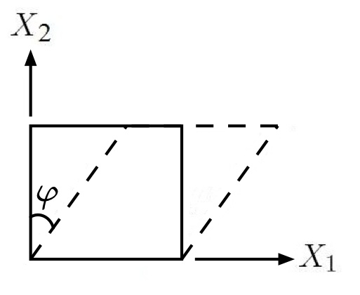
Determine the stress and strain state in a rectangular block, made from the Mooney-Rivlin material of e.x. 1, under simple shear of amount $\varphi$ , in the direction $X_1$ :

$\boldsymbol{\sigma}=-\rho_0 \mathbf{I}+2\left[\underbrace{(\frac{1}{2}+\beta)\frac{\mu}{2}}_{a}\mathbf{B}-\underbrace{(\frac{1}{2} - \beta)\frac{\mu}{2}}_{b}\mathbf{B}^{-1}\right]$ (from the previous e.x)

If $k=tan\varphi$ , $\quad x_1=X_1+kX_2 ; x_2=X_2 ; x_3=X_3 ; \sigma_{33}=0$

We can easily calculate $\mathbf{F}$ and $\mathbf{B}$ :

$\mathbf{F}=\begin{bmatrix}1 & k & 0\\0 & 1 & 0\\0 & 0 & 1 \end{bmatrix}$

$\mathbf{B}=\mathbf{F} \cdot \mathbf{F}^{T}=\begin{bmatrix}k^2+1 & k & 0\\k & 1 & 0\\0 & 0 & 1\end{bmatrix}$
$\mathbf{B}^{-1}=\begin{bmatrix}1 & -k & 0\\-k & 1+k^2 & 0\\0 & 0 & 1\end{bmatrix}$
note: $\mathbf{E}=\begin{bmatrix}0 & \frac{1}{2}k & 0\\\frac{1}{2}k & \frac{1}{2}k^2 & 0\\0 & 0 & 0\end{bmatrix}$

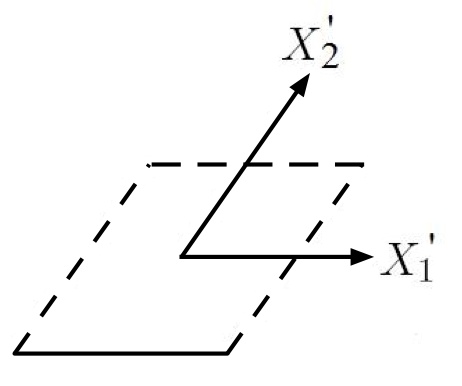
Let’s take a moment to look at the figure below. Aside from $\mathbf{B}$ being defined in spatial coordinates, it’s also “Eulerian” and thus is more difficult to interpret, physically, for most engineers. From inspection of $\mathbf{E}$ , however, we can see that the coordinate system must be deformed, as shown in the figure below, otherwise $E_{22}$ would be zero.

This is mentioned now because the next topic is rate forms, where it is commonly assumed (simplified) that the bases are orthogonal, which can lead to dubious results where large shear deformation is present.

note: both $\sigma_{11}$ and $\sigma_{22}$ are nonzero but it is common to have stress without strain for an incompressible material

$\sigma_{11}=-\rho_0+2a*(\underbrace{1+k^2}_{B_{11}})-2b*(\underbrace{1}_{[B^{-1}]_{11}})$
$\sigma_{22}=-\rho_0+2a*(\underbrace{1}_{B_{22}})-2b*(\underbrace{1+k^2}_{[B^{-1}]_{22}})$

$\sigma_{12}=2(a+b)k \longleftarrow$ no $\rho_0$ because $\rho I_{12}=0$ due to $\mathbf{I}$ being a diagonal matrix
$\sigma_{33}=-\rho_0+2a-2b$
$\sigma_{23}=0$
$\sigma_{31}=0$

$\sigma_{33}=0 \longrightarrow -\rho_0+2a-2b=0 \longrightarrow \rho_0=2(a-b)$
(substitute into the above expressions)

$\sigma_{11}=2ak^2 \quad \sigma_{22}=-2bk^2 \quad \sigma_{12}=2(a+b)k$

note: $k=tan\varphi=\varphi$ for infinitesimal strains $\rightarrow \varphi^{2} << \varphi \rightarrow \sigma_{11}$ and $\sigma_{22}$ may become negligible

note: $\mathbf{E}$ and $\mathbf{e}$ both approach $\begin{bmatrix}0 & k & 0\\k & 0 & 0\\0 & 0 & 0\end{bmatrix}$ for infinitesimal strain, but they would not be equal if large rigid body rotations were present

In summary, an axial test gives $\sigma_{11}$ and “ $\lambda_1$ ” while a shear test gives you $\sigma_{12}$ and “ $k$ .” Once these data are known, then there are two equations in $\sigma_{11}$ , $\sigma_{12}$ and one can solve for the two unknowns: $\mu$ and $\beta.$ It is also possible to obtain the same information from a pure shear test (rather than a simple shear test). Note that it is often easier, in practice, to perform a so-called planar tension test, which would give the same information as a pure shear test, as long as the specimen is incompressible [Bergstrom].

Note that is is possible to obtain $\mu$ and $\beta$ using many other approaches, as these two values are not unique, even for a particular rubber material. For example, since the Mooney-Rivlin model is nonlinear (as is the rubber material of interest, most likely), simply using two stress-strain pairs from the uniaxial test would result in two equations, from which $\mu$ and $\beta$ can be obtained. In reality, a single uniaxial test (or simple shear test) gives a very large number of stress-strain pairs, and the Mooney-Rivlin model fit will depend on which pairs are chosen, none of which will provide a perfect fit. Keep in mind that the goal is not necessarily to obtain the best possible fit to a given set of data (from a particular material test, for example). More often, the goal is to calibrate the material model so that it will give reasonable results under any possible kind of loading.

Yeoh Rubber

The following is known as the Yeoh strain energy function [Yeoh]:

$\begin{equation*} \phi=c_{1} (I_B-3)+c_{2} (I_B-3)^2+c_{3} (I_B-3)^3 \end{equation*}$

The Yeoh function is worth mentioning because it depends only on the first invariant of strain, $I_B$ , unlike the Mooney-Rivlin model, which we recall was a function of both $I_B$ and $II_B$ . Most elastomers (in particular the carbon-filled ones) depend primarily on $I_B$ [Bergstrom] [Holzapfel], and it turns out that the Yeoh model is able to simulate the general behavior of such elastomers even better than the Mooney-Rivlin model [Bergstrom].

The other interesting characteristic of the Yeoh model is that it requires the determination of three constants, compared to the two required in the Mooney-Rivlin model. One option for characterizing the Yeoh model would be to perform the same two tests described above for the Mooney-Rivlin model, and perform a third test – a biaxial tension test – in order to obtain the three Yeoh constants. A uniaxial compression test gives the same information as the biaxial tension test for an incompressible material, so that is another viable alternative [Bergstrom].

We can certainly obtain the three Yeoh constants by simply using three stress-strain pairs from a single test. The question is whether the model would be accurate. It turns out that performing three distinct materials tests in order to characterize the hyperelastic behavior of a material is often not necessary, especially when using models like the Yeoh model, which depend only on the first invariant. In the event that the Yeoh model shall be characterized (all three constants determined) from a single stress-strain pair in a uniaxial test (as is often done in practice), [Bergstrom] states that $c_{2} \approx -0.01c_{1}$ and $c_{3} \approx -0.01c_{2}$ can be assumed. In the case study in the next section (Section 6: Tabulated and Calibrated Models), we’ll see that those two simplified relations are indeed a good rule-of-thumb.

Blatz-Ko Foam

Consider the following strain energy function, which is a simplified version of the Blatz-Ko function [Blatz]:

note: It has been assumed that the material is compressible, with a Poisson Ratio $\nu=.25$

$\begin{equation*} \phi=\frac{1}{2}\mu\left(2III_B^{1/2}+II_BIII_B^{-1}-5\right) \end{equation*}$

We can derive the constitutive equation for $\boldsymbol{\sigma}$ in terms of $\mu$ and $\mathbf{B}$ as follows:

$\frac{\partial \phi}{\partial I_B}=0$
$\frac{\partial \phi}{\partial II_B}=\frac{1}{2} \mu III_B^{-1}$
$\frac{\partial \phi}{\partial III_B}=\frac{1}{2} \mu (III_B^{-1/2}-II_BIII_B^{-2})$

Substituting into eq. 9 in Section 6: Hyperelasticity, re-written below:

$\begin{equation*} \boldsymbol{\sigma}=\frac{2}{det\mathbf{B}^{1/2}}\left[(III_B\frac{\partial \phi}{\partial III_B}+\frac{\partial \phi}{\partial II_B}II_B)\mathbf{I}+\frac{\partial \phi}{\partial I_B}\mathbf{B}-III_B\frac{\partial \phi}{\partial II_B}\mathbf{B}^{-1}\right] \end{equation*}$

We then get:

$\boldsymbol{\sigma}=\frac{2}{det\mathbf{B}^{1/2}}\bigg[\left(III_B*\frac{1}{2} \mu (III_B^{-1/2}-II_BIII_B^{-2})+\frac{1}{2} \mu III_B^{-1}*II_B\right)\mathbf{I}$
$-III_B*\frac{1}{2} \mu III_B^{-1}*\mathbf{B}^{-1}\bigg]$

This reduces to:

$\begin{equation*} \boldsymbol{\sigma}=\frac{1}{det\mathbf{B}^{1/2}}*\mu(III_B^{1/2}\mathbf{I}-\mathbf{B}^{-1}) \end{equation*}$

$\begin{equation*} \boldsymbol{\sigma}=\mu\left(\mathbf{I}-III_B^{-1/2}\mathbf{B}^{-1}\right) \end{equation*}$

$\mu$ is analogous to the “shear modulus” as we’ll see in linear infinitesimal elasticity in a later chapter. However, in order to simplify experimentation, a simple uniaxial test is often performed in order to determine $\mu$ for materials that follow the above Blatz-Ko function.

A more general, compressible, Blatz-Ko function is given in [Holzapfel].

Arruda-Boyce Rubber

Before we get to the Ogden rubber model, which will be discussed at length in this section and the next one, let’s briefly describe the Arruda-Boyce model [Arruda]. The Arruda-Boyce model, sometimes called the “Eight-Chain model” is a very popular model and, along with the Ogden model, is a function of the so-called “principal stretches.” Unlike all of the previous models, which are “phenomenological,” the Arruda-Boyce model is “micromechanical.” It is a statistically derived model based on the macromolecular physical mechanics of “long-chain” materials. The strain energy density function is given as:

$\begin{align*} \phi & = nk\Theta\left[\frac{1}{2}(I_B-3)+\frac{1}{20N}(I_B^2-9)+\frac{11}{1050N^2}(I_B^3-27)\right]\\ & + nk\Theta\left[\frac{19}{7000N^3}(I_B^4-81)+\frac{519}{673750N^4}(I_B^5-243)\right]+\frac{K}{2}(III_B-1)^2 \end{align*}$

$nk\Theta$ are, respectively, the “chain density,” Boltzmann’s constant, and temperature, and as a product represent the shear modulus, $G$ .
$I_B$ is related to the stretch in the “polymer chain.” [Holzapfel]

Note that the last term in the Arruda-Boyce strain energy density function goes to zero for incompressible (“rubbery”) material. We can also see that the Arruda-Boyce rubber model depends only on the principal stretches – i.e. we can substitute $I_B = \lambda_{1}^2+\lambda_{2}^2+\lambda_{3}^2$ into the above equation, where $\lambda_{1}$ , $\lambda_{2}$ , and $\lambda_{3}$ are the eigenvalues of the Left Stretch Tensor, $\mathbf{V}$ , or the Right Stretch Tensor, $\mathbf{U}$ . Recall that $\mathbf{V}$ and $\mathbf{U}$ have the same eigenvalues and the same invariants, but different eigenvectors. The $\lambda$ are commonly called the principal stretches, and usually refer to the eigenvalues along the principal axes of $\mathbf{V}$ . To find a constitutive relationship for the Cauchy Stress, $\boldsymbol{\sigma}$ , we could use the following relationship (derived in Appendix C.3, or alternatively, in Ogden’s textbook):

$\begin{equation*} \sigma_i=\underbrace{\frac{1}{\lambda_{j}\lambda_{k}}}_{\text{no sum}}\frac{\partial{\phi}}{\partial{\lambda_{i}}} \end{equation*}$

$\sigma_i$ are the principal true stresses (the eigenvalues of the Cauchy Stress, $\boldsymbol{\sigma}$ ).

Alternatively, for incompressibility, and where $\phi$ is only a function of $I_\mathbf{B}$ (for the general incompressible relation, see Ogden’s textbook), we have:

$\begin{equation*} \sigma_i=-p+\frac{1}{\cancel{III_\mathbf{V}}}\lambda_i\frac{\partial\phi}{\partial I_\mathbf{B}}\frac{\partial I_\mathbf{B}}{\partial \lambda_i} \end{equation*}$

where “ $p$ ” is our “hydrostatic” term that would need to be found from boundary conditions and $III_\mathbf{V} \approx 1$ .

Since $\frac{d I_\mathbf{B}}{d \lambda_i}$ is $2\lambda_i$ , we get:

(2) $\begin{equation*} \sigma_i=-p+2\lambda_i^2\frac{\partial\phi}{\partial I_\mathbf{B}} \end{equation*}$

Keep in mind that eq. 2 is only valid if $\phi=\phi(I_\mathbf{B})$ .

The Arruda-Boyce model presented here is the original version [Arruda], and is typically used to describe soft, carbon-filled, elastomers at large strains. Other versions of this model exist [Bergstrom] [PolyUMod] that are more suitable for describing the behavior of elastomers in the smaller strain range (less than 30%). This kind of behavior is most often of interest for relatively stiff polymers.

That’s all that will be said about the Arruda-Boyce model. What we will do in the remainder of this section is derive the constitutive expression for the Ogden model, which we will need in order to form our “tabulated” constitutive relationship in the next section, which will be based on the Ogden model.

Ogden Rubber

The strain energy density function for an Ogden material [Ogden], is given by

(3) $\begin{equation*} \phi=\sum_{n=1}^3 \sum_{s=1}^m \frac{\mu_s}{\alpha_s}(\lambda_n^{*\alpha_s}-1)+K(III_\mathbf{V}-1-\ln III_\mathbf{V}) \end{equation*}$

In eq. 3, $\mu_s$ and $\alpha_s$ are material constants.
$\lambda_n^*=\lambda_n*III_\mathbf{V}^{-1/3}$ and $III_\mathbf{V}=\lambda_1\lambda_2\lambda_3$
Eq. 3 is valid for nearly incompressible materials.

The strain energy density function, $\phi$ , for the Ogden model will be a function of the principal stretches, just as in the Arruda-Boyce model. We will make use of the constitutive relationship:

(4) $\begin{equation*} \sigma_i=\underbrace{\frac{1}{\lambda_j \lambda_k}}_{\text{no sum}}\frac{\partial{\phi}}{\partial{\lambda_i}} \end{equation*}$

Eq. 4 is derived in Appendix C.3.

[Holzapfel] shows an equivalent relation in terms of the Second Piola-Kirchhoff stress.

To derive the Ogden constitutive relationship, we need to find $\frac{\partial{\phi}}{\partial{\lambda_i}}$ for the Ogden strain energy density function.

In the following derivation, $i$ , $j$ , $k$ , will be used as subscripts to indicate eigenvalues $1$ , $2$ , $3$ . Unless indices are repeated, they should not be summed.

$\frac{\partial\left({\sum_{n=1}^3\frac{\mu_s}{\alpha_s}\lambda_n^{*\alpha_s}}\right)}{\partial{\lambda_i}}=\frac{\partial\left({\sum_{n=1}^3\frac{\mu_s}{\alpha_s}\lambda_n^{\alpha_s}}III_\mathbf{V}^{-\frac{\alpha_s}{3}}\right)}{\partial{\lambda_i}}=\overbrace{\frac{\mu_s\alpha_s\lambda_i^{\alpha_s-1}}{\alpha_s}III_\mathbf{V}^{-\frac{\alpha_s}{3}}}^{\text{only one term since} \frac{\partial{\lambda_n^{\alpha_s}}}{\partial{\lambda_i}}=\delta_{in}}$ $+\overbrace{\sum_{n=1}^3\frac{\mu_s\lambda_n^{\alpha_s}}{\alpha_s}(-\frac{\alpha_s}{3})III_\mathbf{V}^{(-\frac{1}{3}\alpha_s-1)}\underbrace{\lambda_j\lambda_k}_{\text{no sum}}}^{\text{3 terms since nonzero for all values of n}}$
$=\mu_s\frac{\lambda_i^{\alpha_s}}{\lambda_i}III_\mathbf{V}^{-\frac{\alpha_s}{3}}-\sum_{n=1}^3\mu_s\frac{\lambda_n^{\alpha_s}}{3}III_\mathbf{V}^{(-\frac{1}{3}\alpha_s-1)}\underbrace{\lambda_j\lambda_k}_{\text{no sum}}$

(5) $\begin{equation*} \frac{\partial({\sum_{n=1}^3\frac{\mu_s}{\alpha_s}\lambda_n^{*\alpha_s}})}{\partial{\lambda_i}}=\mu_s\frac{\lambda_i^{*\alpha_s}}{\lambda_i}-\sum_{n=1}^3\mu_s\frac{\lambda_n^{*\alpha_s}}{3}III_\mathbf{V}^{-1}\underbrace{\lambda_j\lambda_k}_{\text{no sum}} \end{equation*}$

$\frac{\partial{K(III_\mathbf{V}-\ln III_\mathbf{V})}}{\partial \lambda_i}=K(\frac{\partial III_\mathbf{V}}{\partial \lambda_i}-\frac{\partial \ln{ III_\mathbf{V}}}{\partial \lambda_i})=K(\overbrace{\lambda_j \lambda_k}^{\text{no sum}}-\frac{1}{III_\mathbf{V}}\overbrace{\lambda_j \lambda_k}^{\text{no sum}})$

(6) $\begin{equation*} \frac{\partial{K(III_\mathbf{V}-\ln III_\mathbf{V})}}{\partial \lambda_i}=K\overbrace{\lambda_j \lambda_k}^{\text{no sum}}\frac{(III_\mathbf{V}-1)}{III_\mathbf{V}} \end{equation*}$

eq. 5 and eq. 6 $\longrightarrow$ eq. 4, where $\phi$ is given by the Ogden formula (eq. 3), yields the following result:

(7) $\begin{equation*} \sigma_i=\sum_{s=1}^m\frac{\mu_s}{III_\mathbf{V}}\left[\lambda_i^{*\alpha_s}-\sum_{n=1}^3\frac{\lambda_n^{*\alpha_s}}{3}\right]+K\frac{III_\mathbf{V}-1}{III_\mathbf{V}} \end{equation*}$

Three or more pairs of experimental constants ( $m \geq 3$ ) in the Ogden model will result in a model that gives excellent behavior over a wide range of strains. Typical values of constants are provided in [Holzapfel].

Among the phenomenological models, the Ogden and Blatz-Ko models are good choices for nearly incompressible, unfilled, rubbers, or foams (respectively). [Holzapfel] shows that the Mooney-Rivlin model is really a special case that can be derived from either the Ogden model or the Blatz-Ko model (note: only the simplified Blatz-Ko model was presented above). In Ogden’s Non-linear Elastic Deformations textbook, he demonstrates that all three of these models can be derived from a general strain energy density function if it is written as an infinite power series. The Mooney-Rivlin model (Eq. 1), for example, ignores all but two of the terms in this power series.

The volumetric parts of these polymer models are often decoupled in FEA codes. Re-writing these models in their decoupled forms is also a useful way to see that they are all really of a similar form. This is illustrated nicely in [Holzapfel].

Sample Python code for all of these material models is provided with the purchase of the textbook “Mechanics of Solid Polymers” [Bergstrom].

J. Bergstrom, PolyUMod User’s Manual, v.1.8.7 ed., Needham, MA: Veryst Engineering, LLC, 2009.
[Bibtex]

@BOOK{PolyuMod,
    Address        = {Needham, MA},
    Author         = {Jorgen Bergstrom},
    Edition        = {v.1.8.7},
    Publisher      = {Veryst Engineering, LLC},
    Title          = {PolyUMod User's Manual},
    Year           = {2009}
}

P. J. Blatz and W. L. Ko, “Application of Finite Elastic Theory to the Deformation of Rubbery Materials,” Transactions of the Society of Rheology, vol. 6, iss. 1, pp. 223-252, 1962.
[Bibtex]

@article{Blatz,
author = {Paul J. Blatz and William L. Ko},
collaboration = {},
title = {Application of Finite Elastic Theory to the Deformation of Rubbery Materials},
publisher = {SOR},
year = {1962},
journal = {Transactions of the Society of Rheology},
volume = {6},
number = {1},
pages = {223-252},
doi = {10.1122/1.548937}
}

E. M. Arruda and M. C. Boyce, “A three-dimensional constitutive model for the large stretch behavior of rubber elastic materials,” Journal of the Mechanics and Physics of Solids, vol. 41, iss. 2, pp. 389-412, 1993.
[Bibtex]

@article{Arruda,
title = "A three-dimensional constitutive model for the large stretch behavior of rubber elastic materials",
journal = "Journal of the Mechanics and Physics of Solids",
volume = "41",
number = "2",
pages = "389 - 412",
year = "1993",
note = "",
issn = "0022-5096",
doi = "DOI: 10.1016/0022-5096(93)90013-6",
author = "Ellen M. Arruda and Mary C. Boyce"
}

M. Mooney, “A Theory of Large Elastic Deformation,” Journal of Applied Physics, vol. 11, iss. 9, pp. 582-592, 1940.
[Bibtex]

@ARTICLE{Mooney,
author={Mooney, M.},
journal={Journal of Applied Physics},
title={A Theory of Large Elastic Deformation},
year={1940},
month={sep },
volume={11},
number={9},
pages={582 -592},
keywords={},
doi={10.1063/1.1712836},
ISSN={0021-8979},}

R. S. Rivlin, “Large Elastic Deformations of Isotropic Materials. I. Fundamental Concepts,” Philosophical Transactions of the Royal Society of London. Series A, Mathematical and Physical Sciences, vol. 240, iss. 822, p. pp. 459-490, 1948.
[Bibtex]

@article{Rivlin,
     jstor_articletype = {research-article},
     title = {Large Elastic Deformations of Isotropic Materials. I. Fundamental Concepts},
     author = {Rivlin, R. S.},
     journal = {Philosophical Transactions of the Royal Society of London. Series A, Mathematical and Physical Sciences},
     jstor_issuetitle = {},
     volume = {240},
     number = {822},
     jstor_formatteddate = {Jan. 13, 1948},
     pages = {pp. 459-490},
     ISSN = {00804614},
     abstract = {},
     language = {English},
     year = {1948},
     publisher = {The Royal Society},
     copyright = {Copyright � 1948 The Royal Society},
}

R. W. Ogden, “Large Deformation Isotropic Elasticity – On the Correlation of Theory and Experiment for Incompressible Rubberlike Solids,” Proceedings of the Royal Society of London. A. Mathematical and Physical Sciences, vol. 326, iss. 1567, pp. 565-584, 1972.
[Bibtex]

@article{Ogden,
author = {Ogden, R. W.},
title = {Large Deformation Isotropic Elasticity - On the Correlation of Theory and Experiment for Incompressible Rubberlike Solids},
volume = {326},
number = {1567},
pages = {565-584},
year = {1972},
doi = {10.1098/rspa.1972.0026},
journal = {Proceedings of the Royal Society of London. A. Mathematical and Physical Sciences}
}

J. S. Bergstrom and M. C. Boyce, “Mechanical behavior of particle filled elastomers,” Rubber chemistry and technology, vol. 72, p. pp. 633�656, 1999.
[Bibtex]

@article{Bergstrom,
     jstor_articletype = {research-article},
     title = {Mechanical behavior of particle filled elastomers},
     author = "Jorgen S. Bergstrom and Mary C. Boyce",
     journal = {Rubber chemistry and technology},
     jstor_issuetitle = {},
    volume = {72},
     pages = {pp. 633�656},
     abstract = {},
     language = {English},
     year = {1999},
     publisher = {American Chemical Society},
}

O. H. Yeoh, “Some forms of the strain energy function for rubber,” Rubber Chem. Technol., vol. 66, iss. 5, pp. 754-771, 1993.
[Bibtex]

@ARTICLE{Yeoh,
author={Yeoh, O.H.},
journal={Rubber Chem. Technol.},
title={Some forms of the strain energy function for rubber},
year={1993},
volume={66},
number={5},
pages={754 -771},
keywords={},
}

G. Holzapfel, Nonlinear Solid Mechanics, John Wiley & Sons Ltd., England, 2000.
[Bibtex]

@book{Holzapfel,
  title={Nonlinear Solid Mechanics},
  author={Holzapfel, GA},
  year={2000},
  publisher={John Wiley \& Sons Ltd., England}
}

J. Bergstrom, Mechanics of Solid Polymers: Theory and Computational Modeling, William Andrew, 2015.
[Bibtex]

@book{Bergstrom_book,
  title={Mechanics of {S}olid {P}olymers: {T}heory and {C}omputational {M}odeling},
  author={Bergstrom, Jorgen},
  volume={},
  year={2015},
  publisher={William Andrew}
}

R. W. Ogden, Non-linear elastic deformations, Dover, 1997.
[Bibtex]

@book{Ogdenbook,
  title={Non-linear elastic deformations},
  author={Ogden, Raymond W},
  year={1997},
  publisher={Dover}
}

Next: 6. Tabulated and Calibrated Models

Leave a Reply Cancel reply