Polar Decomposition

Any matrix can be decomposed into a sum of symmetric and antisymmetric matrices, but $\mathbf{F}$ can be decomposed into a product of two matrices (one symmetric and one orthogonal)

(1) $\begin{equation*} \mathbf{F=V \cdot R = R \cdot U} \end{equation*}$

$\mathbf{U}$ and $\mathbf{V}$ are called the Right Stretch Tensor and Left Stretch Tensor due to their respective positions (relative to $\mathbf{R}$ ) in eq. 1.

$\mathbf{V}=\mathbf{V}^{T}$ (symmetric)
$\mathbf{U}=\mathbf{U}^{T}$ (symmetric)
$\mathbf{R}^{T}=\mathbf{R}^{-1}$ (orthogonal)

A proof of the orthogonality of $\mathbf{R}$ is given in Appendix A.3.

(2) $\begin{equation*} \mathbf{C=F}^{T} \cdot \mathbf{F=U \cdot} \underbrace{\mathbf{R}^{T} \cdot \mathbf{R}}_{\mathbf{I}} \cdot \mathbf{U=U}^{2} \end{equation*}$

(3) $\begin{equation*} \mathbf{B=V}^{2} \end{equation*}$

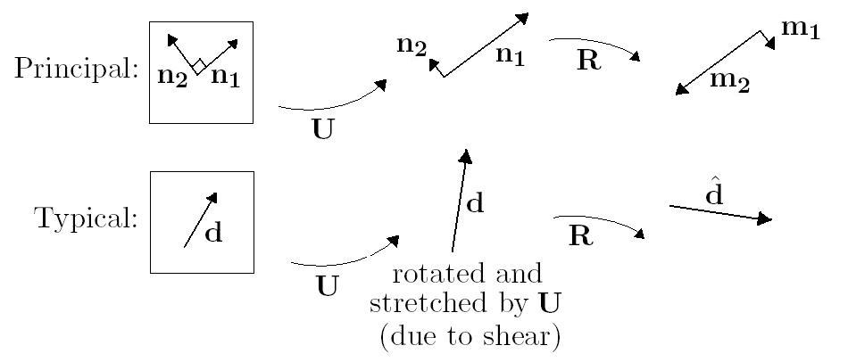
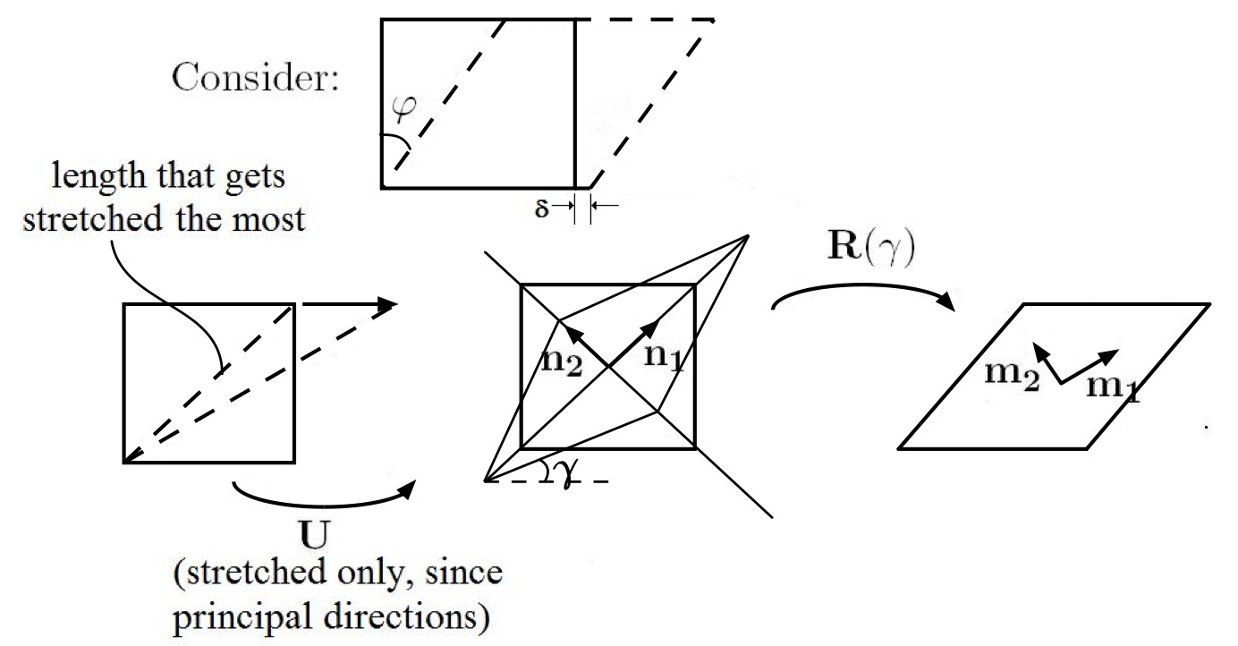
$\mathbf{R}$ is a rigid body rotation, while $\mathbf{U}$ or $\mathbf{V}$ each stretch and rotate (they each contain both normal and shear deformations, typically)

$\mathbf{U}$ and $\mathbf{V}$ have the same eigenvalues. Eigenvalues do not have an “order,” per se, but since $\mathbf{U}$ and $\mathbf{V}$ typically have different eigenvectors, one should be cautious when assuming equivalency of eigenvalues. In the principal directions of $\mathbf{U}$ or $\mathbf{V}$ , $\mathbf{U}$ or $\mathbf{V}$ contains no shear deformation (see Fig). We’ll look at actual stresses, later.

To find the principal directions of $\mathbf{U}$ and $\mathbf{V}$ , we must solve the eigenvalue problem:

$\mathbf{U \cdot n}=\lambda \mathbf{n}$
$\underbrace{\mathbf{R \cdot U}}_{\mathbf{F}} \cdot \mathbf{n}=\mathbf{R \cdot}\lambda \mathbf{n}$ (pictured)
$\mathbf{F = V \cdot R} \longrightarrow \mathbf{V \cdot (}\underbrace{\mathbf{R \cdot n}}_{\mathbf{m}})=\lambda (\underbrace{\mathbf{R \cdot n}}_{\mathbf{m}})$
$\mathbf{m_i}=\mathbf{R \cdot n_i}$

e.x. Polar Decomposition

The deformed equilibrium configuration of a body defined by the deformation mapping:

$x_1=X_1+3X_2$ , $x_2=X_2$ , $x_3=X_3$

Determine:

a) $\mathbf{F}$ and $\mathbf{C}$
b) Eigenvalues and eigenvectors of $\mathbf{C}$
c) $\mathbf{U}$ and $\mathbf{U^{-1}}$
d) $\mathbf{R}$
e) $\mathbf{V}$

a) $\mathbf{F}$ = $\begin{bmatrix} \frac{\partial x_1}{\partial X_1} & \frac{\partial x_1}{\partial X_2} & \frac{\partial x_1}{\partial X_3}\\ \frac{\partial x_2}{\partial X_1} & \frac{\partial x_2}{\partial X_2} & \frac{\partial x_2}{\partial X_3}\\ \frac{\partial x_3}{\partial X_1} & \frac{\partial x_3}{\partial X_2} & \frac{\partial x_3}{\partial X_3} \end{bmatrix} = \begin{bmatrix} 1 & 3 & 0\\ 0 & 1 & 0\\ 0 & 0 & 1 \end{bmatrix}$

note: $\mathbf{F}$ will typically be a function of $X_1$ , $X_2$ , $X_3$ and we’ll be interested in the value of $\mathbf{F}$ at a particular point. Here, it doesn’t matter.

$\mathbf{C=F}^{T} \cdot \mathbf{F}=\begin{bmatrix} 1 & 3 & 0\\ 3 & 10 & 0\\ 0 & 0 & 1\end{bmatrix}$

b) $\mathbf{C \cdot n}=\lambda \mathbf{n}$ ; $det|-\lambda \mathbf{I+C}|=0$
$\longrightarrow \lambda_1=.092$ ; $\lambda_2=1$ ; $\lambda_3=10.91$

$[-\lambda_i \mathbf{I+C}]\mathbf{n_i}=0$

i.e. for $\lambda_1$ ,
$.908n_1+3n_2=0$
$3n_1+9.908n_2=0$
$.908n_3=0$

Choose arbitrary $n_1$ ; solve for $n_2$ from either equation ; normalize:

$\begin{bmatrix}n_1 \\ n_2 \\ n_3\end{bmatrix}_{\lambda_1} = \begin{bmatrix}.957 \\ -.290 \\ 0 \end{bmatrix} ; \begin{bmatrix}n_1 \\ n_2 \\ n_3 \end{bmatrix}_{\lambda_2} = \begin{bmatrix} 0 \\ 0 \\ 1 \end{bmatrix} ; \begin{bmatrix}n_1 \\ n_2 \\ n_3 \end{bmatrix}_{\lambda_3} = \begin{bmatrix}.290 \\ .957\\ 0 \end{bmatrix}$

c) $[\mathbf{U}]_{\mathbf{n}}=\sqrt{[\mathbf{C}]_{\mathbf{n}}}=\begin{bmatrix}\sqrt{\lambda_1} & & \\& \sqrt{\lambda_2} & \\ & & \sqrt{\lambda_3}\end{bmatrix}=\begin{bmatrix}.303 & & \\& 1 & \\ & & 3.303\end{bmatrix}$

$[\mathbf{U}]_{\mathbf{e}}=[\boldsymbol{\Phi}][\mathbf{U}]_{\mathbf{n}}[\boldsymbol{\Phi}]^{T}=\begin{bmatrix} .56 & .83 & 0\\.83 & 3.05 & 0\\0 & 0 & 1\end{bmatrix}$ (symmetric)
where $[\boldsymbol{\Phi}]=\begin{bmatrix} (n_1)_{\lambda_1}&(n_1)_{\lambda_2}&(n_1)_{\lambda_3} \\(n_2)_{\lambda_1}&(n_2)_{\lambda_2}&(n_2)_{\lambda_3} \\ (n_3)_{\lambda_1}&(n_3)_{\lambda_2}&(n_3)_{\lambda_3} \end{bmatrix}$

It’s important to keep in mind that $\mathbf{U}$ , $\mathbf{E}$ , and $\mathbf{C}$ have the same eigenvectors and that these eigenvectors (and any other strain direction or magnitude) are generally dependent on the particular point in space of interest (e.g. $\mathbf{X_1}$ , $\mathbf{X_2}$ , $\mathbf{X_3}$ ). For this simple example, $\mathbf{F}$ is independent of $\mathbf{X_1}$ , $\mathbf{X_2}$ , and $\mathbf{X_3}$ (i.e. the deformation is the same everywhere in the body – a “homogenous” deformation), but this would generally not be the case.

The eigenvalues occur in the direction of the eigenvectors, thus, $\mathbf{n_1 \cdot E \cdot n_1}=\lambda_1$ ; $\mathbf{n_2 \cdot E \cdot n_2}=\lambda_2$ ; $\mathbf{n_3 \cdot E \cdot n_3}=\lambda_3$ . It makes sense that if we only know the eigenvectors and want to undo this transformation to bring us back to $\mathbf{E}$ , then we need a transformation matrix that involves $\mathbf{n_1},\mathbf{n_2},\mathbf{n_3}$ . We can see that $\boldsymbol{\Phi} \cdot \mathbf{U} \cdot \boldsymbol{\Phi}^{T}$ is the opposite of the usual $\boldsymbol{\Phi}^{T} \cdot \mathbf{U} \cdot \boldsymbol{\Phi}$ , and without going through the rigorous derivation of why $\Phi_{i1}=(n_1)_{i}$ , $\Phi_{i2}=(n_2)_{i}$ , $\Phi_{i3}=(n_3)_{i}$ , it at least makes some sense intuitively.

d) $[\mathbf{R}]_{\mathbf{e}}=[\mathbf{F}]_{\mathbf{e}}[\mathbf{U}]_{\mathbf{e}}^{T}=\begin{bmatrix} .55 & .83 & 0\\ -.83 & .55 & 0\\0 & 0 & 1\end{bmatrix}$ (orthogonal ; $\mathbf{R}^{T}=\mathbf{R}^{-1})$

e) $[\mathbf{V}]_{\mathbf{e}}=[\mathbf{F}]_{\mathbf{e}}[\mathbf{R}]_{\mathbf{e}}^{T}=\begin{bmatrix}3.05 & .83 & 0\\.83 & .55 & 0\\0 & 0 & 1\end{bmatrix}$

Leave a Reply Cancel reply