Alternative Measures of Stress

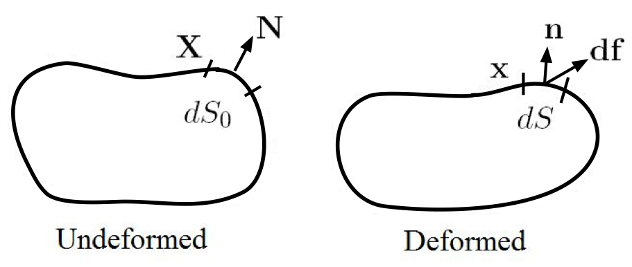
Stress can be defined in the “spatial” coordinate system or in the “material” coordinate system (note that these two coordinate systems differ when rigid body rotation is present). In addition, stress can be defined as force per unit deformed area or force per unit initial area.

$\mathbf{df_n=t_n} \cdot dS$

where $\mathbf{t_n=n} \cdot \boldsymbol{\sigma}$

Now, define $\mathbf{df_n=t_{n}^{0}}dS_0$ , where $\mathbf{t_{n}^{0}=N} \cdot \boldsymbol{\sigma}$
(the actual force, on the undeformed area, gives us the “nominal” stress $\boldsymbol{\sigma}^0$ )

$\mathbf{df_n=t}^0 dS_0=\mathbf{t}dS$

$dS_0\mathbf{N} \cdot \boldsymbol{\sigma}^0=dS\mathbf{n \cdot}\boldsymbol{\sigma}$

Recall Nanson’s Equation (eq. 2 in Section 2: Volume and Area Change): $dS\mathbf{n}=(det\mathbf{F})\mathbf{N} \cdot \mathbf{F}^{-1}dS_0$

$\cancel{dS_0\mathbf{N}} \cdot \boldsymbol{\sigma}^0=(det\mathbf{F})\cancel{dS_0\mathbf{N}} \cdot \mathbf{F}^{-1} \cdot \boldsymbol{\sigma}$

(more formally: $dS_0\mathbf{N} \cdot [\boldsymbol{\sigma}^0-(det\mathbf{F})\mathbf{F}^{-1}\cdot \boldsymbol{\sigma}]=0$ )

(1) $\begin{equation*} \boldsymbol{\sigma}^0=(det\mathbf{F})\mathbf{F}^{-1} \cdot \boldsymbol{\sigma} \end{equation*}$

Eq. 1 is the Nominal Stress Tensor

Now, consider a “pseudo-force” acting in the initial frame of reference (see Fig).

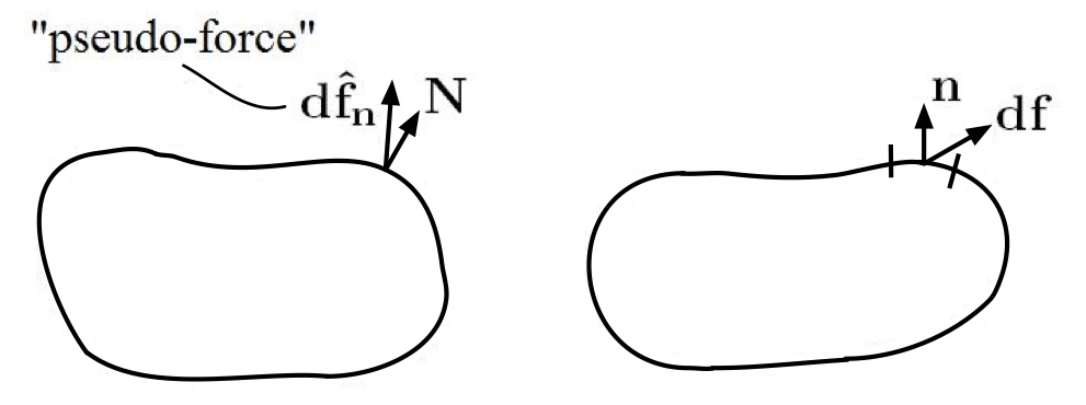
note: The “pseudo-force” pictured in the above figure will become more clear later. The following derivation of the “Second Piola-Kirchhoff” (P-K II) stress tensor is similar to the previous derivation of the “Nominal” stress tensor. The P-K II tensor will be quite useful later on to help us derive constitutive relationships.

Recall $\mathbf{dx=F \cdot dX}$

Similarly, $\mathbf{df_n=F \cdot d\hat{f}_n}$ ; $\mathbf{d\hat{f}_n}=\mathbf{\hat{t}_n}dS_0$ ;
$\mathbf{\hat{t}_n}=\mathbf{N} \cdot \boldsymbol{\hat{\sigma}}$ ; $\boldsymbol{\hat{\sigma}}$ = P-K II tensor

We already know that $\mathbf{df_n=t_n \cdot} dS=\mathbf{n \cdot}\boldsymbol{\sigma}dS$

So, $\mathbf{df_n=F \cdot d\hat{f}_n=F \cdot \hat{t}_n}dS_o=\mathbf{\hat{t}_n} \cdot \mathbf{F}^{T}dS_0=\mathbf{N} \cdot \boldsymbol{\hat{\sigma}} \cdot \mathbf{F}^{T}dS_0$

Substituting for $\mathbf{df_n}$ , $\mathbf{n \cdot}\boldsymbol{\sigma}dS=\mathbf{N \cdot}\boldsymbol{\hat{\sigma}} \cdot \mathbf{F}^{T}dS_o$ (1)

Invoke Nanson’s equation: $\mathbf{n}dS=(det\mathbf{F})\mathbf{N} \cdot \mathbf{F}^{-1}dS_0$ (2)

(2) $\longrightarrow$ (1) $\longrightarrow$ $(det\mathbf{F})\cancel{\mathbf{N}dS_0} \cdot \mathbf{F}^{-1} \cdot \boldsymbol{\sigma}=\cancel{\mathbf{N}dS_0} \cdot \boldsymbol{\hat{\sigma}} \cdot \mathbf{F}^{T}$
(more formally, $\mathbf{N}dS_0 \cdot [(det\mathbf{F})\mathbf{F}^{-1} \cdot \boldsymbol{\sigma}-\boldsymbol{\hat{\sigma}} \cdot \mathbf{F}^{T}]=0$ )

(2) $\begin{equation*} \longrightarrow \boldsymbol{\hat{\sigma}}=(det\mathbf{F})\mathbf{F}^{-1} \cdot \boldsymbol{\sigma} \cdot \mathbf{F}^{-T} \end{equation*}$

Eq. 2 is the $2^{nd}$ Piola-Kirchhoff Stress Tensor

For infinitesimal deformation (ignoring rigid body rotations):
$\mathbf{F} \approx \mathbf{I}$ ; $det\mathbf{F}=1$ ; $\boldsymbol{\sigma} \approx \boldsymbol{\sigma^0} \approx \boldsymbol{\hat{\sigma}}$

e.x. The deformed equilibrium configuration of a body is defined by the deformation mapping:

$x_1=-\frac{1}{2}X_1$ , $x_2=\frac{1}{2}X_3$ , $x_3=2X_2$
(Very large deformations and very large rigid body motions)

The Lagrangian Strain is:

$\mathbf{E}=\frac{1}{2}(\mathbf{F}^{T}\mathbf{F}-\mathbf{I})=\begin{bmatrix}-.375 & 0 & 0\\0 & 1.5 & 0\\0 & 0 & -.375\end{bmatrix}$

$\mathbf{e}=\frac{1}{2}(\mathbf{I}-\mathbf{F}^{-T}\mathbf{F}^{-1})=\begin{bmatrix}-1.5 & 0 & 0\\0 & -1.5 & 0\\0 & 0 & .375\end{bmatrix}$

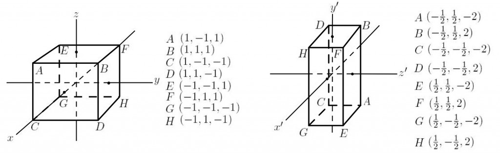
Note that $E_{22}=1.5$ (this is the “ $2$ ” direction ; initially the “ $y$ ” direction). The specimen did not elongate from left to right, yet $E_{22}$ is a positive value. In addition, $E_{11}$ and $E_{33}$ are the same, confirming that they represent the transverse strains. The axes actually underwent a large rigid body rotation. $\mathbf{E}$ is a strain measure that rotates with the axes. In other words, $\mathbf{E}$ is invariant to rigid body rotations. This will be essential to remember in the later chapters!

The Cauchy Stress is:

$\boldsymbol{\sigma}=\begin{bmatrix}0 & 0 & 0\\0 & 0 & 0\\0 & 0 & 100\end{bmatrix}$ (ignore units)

Note that $\boldsymbol{\sigma}$ is defined in a different coordinate system than $\mathbf{E}$ (“spatial” axes rather than “material” axes). $\boldsymbol{\sigma}$ changes with rigid body rotation, while $\mathbf{E}$ does not!

a) Determine the nominal and P-K II stress tensors
b) The nominal and P-K II tractions associated with the plane $x_3$ = $const$ in the undeformed state
c) Repeat parts “a” and “b” for the mapping:
$x_1=-.99X_1$ ; $x_2=.99X_3$ ; $x_3=.99X_2$ (small deformations with very large rigid body motions)

a) and b):

Since the deformations are given, we first find $\mathbf{F}$ :

$\mathbf{F}=\begin{bmatrix}\frac{\partial x_1}{\partial X_1} & \frac{\partial x_1}{\partial X_2} & \frac{\partial x_1}{\partial X_3}\\ \frac{\partial x_2}{\partial X_1} & \frac{\partial x_2}{\partial X_2} & \frac{\partial x_2}{\partial X_3}\\ \frac{\partial x_3}{\partial X_1} & \frac{\partial x_3}{\partial X_2} & \frac{\partial x_3}{\partial X_3} \end{bmatrix}=\begin{bmatrix}-\frac{1}{2} & 0 & 0\\0 & 0 & \frac{1}{2}\\0 & 2 & 0\end{bmatrix}$

With $\mathbf{F}$ and $\boldsymbol{\sigma}$ known, we can find $\boldsymbol{\sigma}^0$

$\boldsymbol{\sigma}^0=(det\mathbf{F})\mathbf{F}^{-1} \cdot \boldsymbol{\sigma}=\begin{bmatrix}0 & 0 & 0\\0 & 0 & 25\\0 & 0 & 0\end{bmatrix}$

Remember, this stress is a result of the actual force on the undeformed area.

From Nanson’s Equation (eq. 2 in Section 2: Volume and Area Change),
$dA_0\mathbf{N}=\frac{1}{(det\mathbf{F})}\mathbf{F}^{T} \cdot \mathbf{n}=\frac{1}{.5}\mathbf{F}^{T} \cdot \begin{bmatrix}0\\0\\1\end{bmatrix}=4*\begin{bmatrix}0\\1\\0\end{bmatrix}$ ,
where $\begin{bmatrix}0\\0\\1\end{bmatrix}$ is the normal to the plane $x_3$ = $constant$
Since we know from inspection that $\mathbf{N}=\begin{bmatrix}0\\1\\0\end{bmatrix}$ , we can see that the undeformed area is four times that of the deformed area, hence we expect the nominal stress to be four times smaller that the true (Cauchy) stress, which it is.

We have everything we need in order to find $\boldsymbol{\hat{\sigma}}$ :

$\boldsymbol{\hat{\sigma}}=(det\mathbf{F})\mathbf{F}^{-1} \cdot \boldsymbol{\sigma} \cdot \underbrace{\mathbf{F}^{-T}}_{[\mathbf{F}^{T}]^{-1}}=\begin{bmatrix}0 & 0 & 0 \\0 & 12.5 & 0\\ 0 & 0 & 0\end{bmatrix}$

Traction on the plane $x_3$ = $constant$ :

$\mathbf{\hat{t}}=\boldsymbol{\hat{\sigma}} \cdot \mathbf{N}=\begin{bmatrix}0 & 0 & 0\\0 & 12.5 & 0\\0 & 0 & 0 \end{bmatrix}\begin{bmatrix}0 \\ 1 \\0\end{bmatrix}=\begin{bmatrix}0\\-12.5\\0\end{bmatrix}$

c) What about small deformation (still large rigid body rotation)?

$\mathbf{F}=\begin{bmatrix}-.99 & 0 & 0\\0 & 0 & .99\\0 & 1.01 & 0\end{bmatrix}$

$\mathbf{E}=\begin{bmatrix}-.00995 & 0 & 0\\0 & .01005 & 0\\0 & 0 & -.00995\end{bmatrix}$

$\mathbf{e}=\begin{bmatrix}-.01015 & 0 & 0\\0 & -.01015 & 0\\0 & 0 & .00985\end{bmatrix}$

$\boldsymbol{\sigma}^0=\begin{bmatrix}0 & 0 & 0\\0 & 0 & 98\\0 & 0 & 0\end{bmatrix}$ ; $\boldsymbol{\hat{\sigma}}=\begin{bmatrix}0 & 0 & 0\\0 & 97 & 0\\0 & 0 & 0\end{bmatrix}$

Note that $\boldsymbol{\hat{\sigma}}$ gives a good answer for small deformations, and is defined in the same coordinate system as $\mathbf{E}$ !

Note that in FEA, $\mathbf{F}$ is found from deformations without the need to determine analytical formulas that describe the coordinate transformations. To see the way that this is done in FEA, see Finite Element Coordinate Mapping [McGinty].

Perhaps now is a good time to discuss some terminology. A tensor can be defined in the spatial configuration or the material configuration, as we’ve now seen. A tensor that is defined in the material configuration, like the Green-Lagrange strain, $\mathbf{E}$ , is invariant to rigid body rotation (review the above example). Tensors that don’t fit into either category (like the deformation gradient) are not used in constitutive relationships, but are nevertheless important and are sometimes called two-point tensors.

Common synonyms for spatial configuration include: deformed configuration, current configuration.
Common synonym for material configuration: reference configuration.

Tensors that are defined in the spatial configuration, like the Cauchy stress, $\boldsymbol{\sigma}$ , are commonly called objective tensors or observer independent tensors. Even though we know that tensors that are defined in the spatial configuration change their values under rigid body rotation, such tensors are commonly called “frame indifferent tensors” which is a particularly vague term that is avoided in this text.

Perhaps adding to the confusion, a tensor that is defined in the spatial configuration can be obtained by a so-called push-forward of a corresponding material tensor. A tensor that is defined in the material configuration can be obtained by a so-called pull-back of a corresponding spatial tensor.

To avoid any ambiguity, the only terminology that is used in this text to distinguish the different types of tensors is spatial and material, which will often be accompanied by additional detailed explanation regarding the physical meaning of the particular tensor.

Leave a Reply Cancel reply