8. Linear Infinitesimal Elasticity

In hypoelasticity, we took the Cauchy stress, $\boldsymbol{\sigma}$ , and developed a constitutive relationship with the Left-Cauchy Green Strain Tensor, $\mathbf{B}$ . This relationship was quite complicated (eq. 9 in Section 6: Hyperelasticity). Recall also that these tensors were both defined in spatial coordinates, by definition. Then, we derived an even more complicated “hypoelastic” formula (eq. 7 in Section 7: Hypoelasticity) that involved the rate of deformation tensor, $\mathbf{D}$ . Lastly, a simple three-line pseudo-algorithm was given to illustrate how actual FEA (“solid” element) codes handle such “rate-form” constitutive expressions to solve, say, transient dynamic problems involving one or more bodies. We saw that this algorithm works equally nicely for linear infinitesimal elasticity as well.

In terms of both the non-rate form of the constitutive relationship and the rate-form, linear infinitesimal elasticity simplifies things considerably. Recall that the Second Piola Kirchhoff Stress Tensor, $\hat{\boldsymbol{\sigma}}$ , can be used for infinitesimal elasticity (review the example at the end of Section 4: Alternative Measures of Stress). Since $\hat{\boldsymbol{\sigma}}$ is defined in material coordinates, we will develop a constitutive relationship with a strain tensor that is similarly invariant to rigid body rotation, viz., $\mathbf{E}$ .

Some authors instead choose to use the Cauchy stress and the Eulerian strain for the formulation of their linear infinitesimal constitutive expression. We are free to choose either stress-strain pair ( $\boldsymbol{\sigma}\leftrightarrow \mathbf{e}$ or $\hat{\boldsymbol{\sigma}}\leftrightarrow \mathbf{E}$ ) in linear infinitesimal elasticity. We saw previously that our “time-stepping algorithm” was independent of this choice.

In this chapter we’ll take a look only at linear infinitesimal elasticity. If a material is subjected to large strain (even if it is linear) or if a material is nonlinear (even if subjected to small strain), then it should be treated using the approaches developed in the previous chapters on hyperelasticity and hypoelasticity. Just as in our chapter on hyperelasticity, the focus here will be on developing a non-rate constitutive expression that relates stress and strain. In the elastic regime, a wide variety of materials, including most metals, behave linearly.

The theory of linear infinitesimal elasticity was developed independent of hyperelastic theory, with the former being mostly developed, originally, from intuition and experience [Malvern]. Nevertheless, the linear theory can be derived as well, using the same starting assumptions that we used at in the previous hyperelasticity derivation.

Recall $\hat{\boldsymbol{\sigma}}=\frac{d\phi}{d\mathbf{E}}$

Infinitesimal elasticity $\longrightarrow \mathbf{E} \approx \boldsymbol{\epsilon}$ , $\hat{\boldsymbol{\sigma}} \approx \boldsymbol{\sigma}$

note: The linear infinitesimal stress will be denoted by $\boldsymbol{\sigma}$ for the remainder of this chapter. So long as $\boldsymbol{\epsilon}$ and $\boldsymbol{\sigma}$ are work conjugate, we can proceed in deriving our constitutive relationship.

We know the following three expressions to be true as well:

$\boldsymbol{\sigma} = \frac{d\phi}{d\boldsymbol{\epsilon}}$
$\epsilon_{ij}=\frac{1}{2}(\frac{\partial u_{i}}{\partial x_{j}}+\frac{\partial u_j}{\partial x_i})$
$x_i \approx X_i$ (still, $u_i = x_i-X_i$ )

In index notation, $\sigma_{ij}=\frac{d\phi}{d\epsilon_{ij}}$

For linear materials, we can define $\phi$ , using a Taylor expansion, as follows:

$\phi=\phi(\epsilon_{ij})=\underbrace{\phi(0)}_{a_0} + \underbrace{\left(\frac{d\phi}{d\epsilon_{ij}}\right)_0^{\phantom{S}}}_{b_{ij}}\epsilon_{ij}+\frac{1}{2}\underbrace{\left(\frac{d^{2}\phi}{d\epsilon_{ij}d\epsilon_{kl}}\right)_0^{\phantom{S}}}_{\mathcal{C}_{ijkl}}\epsilon_{ij}\epsilon_{kl}$

note: This is a taylor series with higher terms neglected

So, $\phi=a_0+b_{ij}\epsilon_{ij}+\frac{1}{2}\mathcal{C}_{ijkl}\epsilon_{ij}\epsilon_{kl}$

(1) $\begin{equation*} \sigma_{ij}=\frac{d\phi}{d\epsilon_{ij}}=b_{ij}+\frac{1}{2}(\mathcal{C}_{ijkl}+\mathcal{C}_{klij})\epsilon_{kl} \end{equation*}$

note: In eq. 1, $\frac{d}{d\epsilon_{ij}}(\mathcal{C}_{mnkl}\epsilon_{mn}\epsilon_{kl})=\mathcal{C}_{mnkl}(\delta_{mi}\delta_{nj}\epsilon_{kl}+\epsilon_{mn}\delta_{ik}\delta_{jl})$
$=\mathcal{C}_{ijkl}\epsilon_{kl}+\mathcal{C}_{mnij}\epsilon_{mn} \text{ (or }\mathcal{C}_{klij}\epsilon_{kl})$

If there is no initial stress:

(2) $\begin{equation*} b_{ij}=0 \end{equation*}$

Note that the order $\frac{d^2\phi}{d\epsilon_{ij}d\epsilon_{kl}}$ or $\frac{d^2\phi}{d\epsilon_{kl}d\epsilon_{ij}}$ doesn’t matter

(3) $\begin{equation*} \mathcal{C}_{ijkl}=\mathcal{C}_{klij} \end{equation*}$

Eq. 3 $\rightarrow$ Eq. 2 $\rightarrow$ Eq. 1 $\longrightarrow$ $\sigma_{ij}=\mathcal{C}_{ijkl}\epsilon_{kl}$

$\mathcal{C}_{ijkl}$ has $3^4=81$ potential terms ( $9$ x $9$ matrix) to begin with.

Symmetry: $\sigma_{ij}=\sigma_{ji}$ and $\epsilon_{kl}=\epsilon_{lk}$ $\longrightarrow$ 36 terms (6 x 6 matrix)

Symmetry in $\mathcal{C} \rightarrow$ $\mathcal{C}_{ijkl}=\mathcal{C}_{klij}$ (i.e. eq. 3 above)
$\longrightarrow$ 21 constants (general anisotropic)

A plane of symmetry is defined as follows: for every pair of coordinate systems that are mirror images of each other about the plane of symmetry, the elastic constants are the same. A single plane of symmetry reduces the number of independent constants to 13. Orthotropic symmetry (three orthogonal planes of symmetry) reduces the number of independent constants to 9. The proof can be found in [Malvern].

Isotropic $\longrightarrow$ only 2 independent constants

Proof:
Recall $\phi=\frac{1}{2}\mathcal{C}_{ijkl}\epsilon_{ij}\epsilon_{kl}$ (valid outside of isotropy)

note: Since $\phi$ is a function of strain only, path dependence is not considered (i.e. we are still only considering elasticity)

Also note: $\phi$ is quadratic

For isotropy: $\phi=\phi(\boldsymbol{\epsilon})=\phi(I_{\boldsymbol{\epsilon}}, II_{\boldsymbol{\epsilon}}, III_{\boldsymbol{\epsilon}})$
$($ recall that for hyperelastic isotropy, $\phi=\phi(\mathbf{B})=\phi(I_{\mathbf{B}}, II_{\mathbf{B}}, III_{\mathbf{B}})$ $)$

Let’s assume $\phi=a I_{\boldsymbol{\epsilon}}^{2}+b II_{\boldsymbol{\epsilon}}$ , using the following reasoning:

We know that $\phi$ is quadratic. Thus, $\phi$ doesn’t depend on $III_{\boldsymbol{\epsilon}}$ , since $III_{\boldsymbol{\epsilon}}$ is cubic ( $\lambda_1 \lambda_2 \lambda_3$ ). $I_{\boldsymbol{\epsilon}}$ is linear and so is, accordingly, squared, in order to obtain a quadratic. Our resulting $I_{\boldsymbol{\epsilon}}^{2}$ term is also multiplied by a coefficient, $a$ . $II_{\boldsymbol{\epsilon}}=\underbrace{\lambda_1 \lambda_2 + \lambda_2 \lambda_3 + \lambda_1 \lambda_3}_{\textrm{already quadratic}}$ is, similarly, multiplied by a constant, $b$ .

Recall that $(I_{\boldsymbol{\epsilon}})^2 \sim (tr(\boldsymbol{\epsilon}))^{2}$ and $II_{\boldsymbol{\epsilon}}$ is a function of both $(tr(\boldsymbol{\epsilon}))^{2}$ and $tr(\boldsymbol{\epsilon}^{2})$ .

Also recall that $tr(\boldsymbol{\epsilon^{2}})=\epsilon_{ij}\epsilon_{ij}$ , since $\boldsymbol{\epsilon}$ is a symmetric tensor.

$\longrightarrow \phi=\underbrace{a(\epsilon_{ii})(\epsilon_{jj})+b(\epsilon_{ij})(\epsilon_{ij})}_{\text{sum over i,j } 1,2,3}$

$\frac{d\phi}{d\epsilon_{mn}}=a[\epsilon_{ii}\frac{d\epsilon_{jj}}{d\epsilon_{mn}}+\epsilon_{jj}\frac{d\epsilon_{ii}}{d\epsilon_{mn}}]+2b[\frac{d\epsilon_{ij}}{d\epsilon_{mn}}\epsilon_{ij}]$
$=a[\epsilon_{ii}\underbrace{\delta_{jm}\delta_{jn}}_{*}+\epsilon_{jj}\underbrace{\delta_{im}\delta_{in}}_{*}]+2b[\delta_{im}\delta_{jn}\epsilon_{mn}]$

* – note that “ $m$ ” must equal “ $n$ ” in the expression that is multiplied by “ $a$ ” in order to be non-zero.

So, $\frac{d\phi}{d\epsilon_{mn}}=2a\epsilon_{ii}+2b\epsilon_{mn}$

$2a \rightarrow$ “ $\lambda$ ”
$b \rightarrow$ “ $\mu$ ”

Recall $\sigma_{ij}=\frac{d\phi}{d\epsilon_{ij}}$ :

(4) $\begin{equation*} \sigma_{ij}=\lambda\epsilon_{kk}\delta_{ij}+2\mu\epsilon_{ij} \end{equation*}$

In eq. 4, $\lambda$ and $\mu$ are $Lam\acute{e}$ elastic constants. We can see that we have two independent constants, as expected. These constants are determined experimentally, as will be discussed shortly.

The following alternative expression is commonly found in literature on FEA:

(5) $\begin{equation*} \boldsymbol{\sigma}=\boldsymbol{\mathcal{C}}:\boldsymbol{\epsilon} \end{equation*}$

We will see later what $\boldsymbol{\mathcal{C}}$ is, as well as why we use the “ $:$ ” operator.

$\begin{bmatrix} \sigma_{11}\\ \sigma_{22}\\ \sigma_{33}\\ \sigma_{23}\\ \sigma_{31}\\ \sigma_{12}\\ \end{bmatrix} = \begin{bmatrix} \mathcal{C}_{1111} & \mathcal{C}_{1122} & \mathcal{C}_{1133} & \mathcal{C}_{1123} & \mathcal{C}_{1131} & \mathcal{C}_{1112}\\ \mathcal{C}_{2211} & \mathcal{C}_{2222} & \mathcal{C}_{2233} & \mathcal{C}_{2223} & \mathcal{C}_{2231} & \mathcal{C}_{2212}\\ \mathcal{C}_{3311} & \mathcal{C}_{3322} & \mathcal{C}_{3333} & \mathcal{C}_{3323} & \mathcal{C}_{3331} & \mathcal{C}_{3312}\\ \mathcal{C}_{2311} & \mathcal{C}_{2322} & \mathcal{C}_{2333} & \mathcal{C}_{2323} & \mathcal{C}_{2331} & \mathcal{C}_{2312}\\ \mathcal{C}_{3111} & \mathcal{C}_{3122} & \mathcal{C}_{3133} & \mathcal{C}_{3123} & \mathcal{C}_{3131} & \mathcal{C}_{3112}\\ \mathcal{C}_{1211} & \mathcal{C}_{1222} & \mathcal{C}_{1233} & \mathcal{C}_{1223} & \mathcal{C}_{1231} & \mathcal{C}_{1212}\\ \end{bmatrix} \begin{bmatrix} \epsilon_{11}\\ \epsilon_{22}\\ \epsilon_{33}\\ 2\epsilon_{23}\\ 2\epsilon_{31}\\ 2\epsilon_{12}\\ \end{bmatrix}$

note: $\boldsymbol{\mathcal{C}}$ is symmetric in matrix form

Also note: The shear terms are multiplied by “2” because we used symmetry of $\boldsymbol{\epsilon}$ to reduce the 9 x 9 tensor, $\boldsymbol{\mathcal{C}}$ , to a 6 x 6.

The matrix “ $\mathcal{C}_{ijkl}$ ” can be written in “Voigt” notation, “ $\mathcal{C}_{IJ}$ ” as well:

$\begin{bmatrix} \mathcal{C}_{11} & \mathcal{C}_{12} & \mathcal{C}_{13} & \mathcal{C}_{14} & \mathcal{C}_{15} & \mathcal{C}_{16}\\ \mathcal{C}_{21} & \mathcal{C}_{22} & \mathcal{C}_{23} & \mathcal{C}_{24} & \mathcal{C}_{25} & \mathcal{C}_{26}\\ \mathcal{C}_{31} & \mathcal{C}_{32} & \mathcal{C}_{33} & \mathcal{C}_{34} & \mathcal{C}_{35} & \mathcal{C}_{36}\\ \mathcal{C}_{41} & \mathcal{C}_{42} & \mathcal{C}_{43} & \mathcal{C}_{44} & \mathcal{C}_{45} & \mathcal{C}_{46}\\ \mathcal{C}_{51} & \mathcal{C}_{52} & \mathcal{C}_{53} & \mathcal{C}_{54} & \mathcal{C}_{55} & \mathcal{C}_{56}\\ \mathcal{C}_{61} & \mathcal{C}_{62} & \mathcal{C}_{63} & \mathcal{C}_{64} & \mathcal{C}_{65} & \mathcal{C}_{66}\\ \end{bmatrix}$

Using Voigt notation, we can construct the following table:

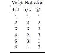
The above table can be simplified in this way due to the symmetries of the $\mathcal{C}_{ijkl}$ tensor apparent upon inspection.

e.g. the way you read the $1^{st}$ row depends on what information you need:

when I = 1, i = 1, j = 1
when J = 1, k = 1, l =1

This is easily confirmed by comparing, say, the “1-1” term in each of the above two matrices.

(6) $\begin{equation*} \mathcal{C}_{ijkl}=\lambda \delta_{ij} \delta_{kl} + \mu (\delta_{ik} \delta_{jl} + \delta_{il} \delta_{jk}) \end{equation*}$

i.e.
$\mathcal{C}_{45}=\underbrace{\mathcal{C}_{2331}}_{\text{Table}}=\lambda \delta_{23} \delta_{31} + \mu(\delta_{23} \delta_{31} + \delta_{21} \delta_{33})=0$

$\mathcal{C}_{44}=\mathcal{C}_{2323}=\lambda \delta_{23} \delta_{23} + \mu(\delta_{22} \delta_{33} + \delta_{23} \delta_{32})=\mu$

note: Eq. 6 is how stiffness matrices are formed in FEA

Sometimes we like to write the constitutive equation in the manner shown in eq. 5. We can prove that this expression is true by noting that the “:” operator is essentially two dot products (it can be easily shown that our previous definition of : for second order tensors still holds true as well).

$\boldsymbol{\sigma}=\underbrace{[\lambda \delta_{ij} \delta_{kl} +\mu (\delta_{ik} \delta_{jl} + \delta_{il} \delta_{jk})]\mathbf{e_i} \otimes \mathbf{e_j} \otimes \mathbf{e_k \otimes e_l}}_{\text{can be thought of as a 9x9 matrix}} : \epsilon_{mn}\mathbf{e_m \otimes e_n}$
$=[\lambda \delta_{ij} \delta_{mn} +\mu (\delta_{im} \delta_{jn} + \delta_{in} \delta_{jm})]\epsilon_{mn}\mathbf{e_i} \otimes \mathbf{e_j}$
$=[\lambda \delta_{ij} \epsilon_{mm} + 2 \mu \epsilon_{ij}]\mathbf{e_i \otimes e_j}$ , which is as expected.

note: symmetry of $\epsilon_{mn}$ was invoked in the last step of the derivation

L. E. Malvern, Introduction to the Mechanics of a Continuous Medium , Upper Saddle River, NJ: Prentice-Hall, Inc. , 1969 .
[Bibtex]

@Book{Malvern,
author = { Malvern, Lawrence. E. },
title = { Introduction to the Mechanics of a Continuous Medium },
isbn = {  },
publisher = { Prentice-Hall, Inc. },
year = { 1969 },
address = {Upper Saddle River, NJ},
}

Leave a Reply Cancel reply